📖 Static Random Utility Models

⏱ | words

References

Static discrete choice model

A decision maker (DM) in state \(x\) chooses an alternative \(d\) from a finite set \(D(x)\) of possible alternatives to maximize utility \(u(x,d)\)

\(\implies\) A decision rule

\[d^*(x) = \arg\max_{d \in D(x)} u(x,d)\]

• If we know the person’s state \(x\), utility function \(u(x,d)\) and choice set \(D(x)\), then we can *perfectly predict the choice \(d^*(x)\) they make

Shifting and scaling utilities of the alternatives

Written as above, the behavioral models has important implications:

1. Only differences in utilities matter \(\iff\) adding an arbitrary constant to \(u(x,d)\) for all \(d\) does not change the choice \(d^*(x)\)

\[d^*(x) =\arg\max_{d \in D(x)} u(x,d) = \arg\max_{d \in D(x)} \big[u(x,d) + \mathrm{const}(x) \big]\]

• This implies that in the non-parametric context utility of one of the alternatives has to be normalized, for example, to zero

• When utility is linear, the constant term for one of the alternatives has to be set to zero

• Also, utility can vary by alternatives, but not by the attributes of DM – which would be identical over the alternatives. The only possibility is cross-effects.

2. The overall scale of the utility is irrelevant \(\iff\) multiplying all utilities by a positive constant does not change the choice \(d^*(x)\)

\[d^*(x) =\arg\max_{d \in D(x)} u(x,d) = \arg\max_{d \in D(x)} \big[ \mathrm{const}(x)\cdot u(x,d) \big], \; \mathrm{const}(x)>0\]

• This has implications for how the variance of the random component of the utility can be treated under different specifications, see below

Probabilistic choice theory

The choice \(d^*\) is not perfectly predictable by the econometrician because DM has private information \(\epsilon\) that affects the choice and that we (as the econometrician) do not observe

\(\implies\) Decision rule is

\[d^*(x,\epsilon)= \arg\max_{d \in D(x)} [u(x,d)+\epsilon(d)]\]

• random variable that is not perfectly predictable

Define the conditional choice probability

\[P(d|x)= \hbox{Prob}\left\{d^*(x,\epsilon)=d|x\right\} = \int_\epsilon I\left\{ d^*(x,\epsilon)=d\right\}q(\epsilon|x) d\epsilon\]

• \(I(\cdot)\) indicator function

• \(g(\epsilon|x)\) pdf of \(\epsilon\) given \(x\)

Development

1. Thurstone [1959] “The measurement of values”

   • Mathematical models of choice in psychology based on stimuli

2. Luce [1959] “Individual choice behavior”

   • Derived logit structure from indepedence of irrelevant alternatives (IIA) property of choice

3. Marschak [1960] “Binary choice constraints and random utility indicators”

   • Showed that this model is consistent with random utility maximization \(\rightarrow\) random utility models (RUM)

4. McFadden [1974] “Conditional logit analysis of qualitative choice behavior”

   • Proved that logit formula for choice probabilities necessarily implies extreme value type I (EV1) distribution of unobservables

Independence of irrelevant alternatives (IIA)

Let \(D(x)\) denote a finite set of alternatives given state \(x\), and \(d\in B \subset D(x)\). The choice model exhibits the IIA property if

\[P(d|x,B) \propto P(d|x,D),\]

where \(P(d|x,A)\) is the choice probability given the choice set \(A\subset D(x)\) and the symbol \(\propto\) denotes proportionality.

The original definition of IIA by Luce [1959] is slightly different, but is equivalent to the above. Let \(P(d_1,d_2)\) denote the probability of choosing \(d_1\) over \(d_2\), and let \(B=\{d_1,d_2\} \subset D(x)\). Luce imposed as IIA

\[ \frac{P(d_1,d_2)}{P(d_2,d_1)} = \frac{P(d_1|x,B)}{P(d_2|x,B)}, \; \forall B \in D(x) \]

Luce Theorem

If IIA holds, then there exist non-negative weights \(v(x,d)\), \(d \in D(x)\) such that

\[P(d|x) = \frac{\exp v(d,x)}{\sum_{d' \in D(x)} \exp v(d',x)}\]

• Luce theorem gives logit structure to the choice probabilities without any specification of \(v(d,x)\)!

I have worked in the highly probabilistic area of psychophysical theory; but the empirical materials have lead me away from axiomatic structures, such as the choice axiom, to more structural, neural models which are not easily axiomatized at the present time. After some attempts to apply choice models to psychophysical phenomena I was lead to conclude that it is not a very promising approach to these data – Luce

Extreme value distribution

Luce’s structure obtains form RUM when unobserved factors \(\epsilon\) have specific distribution

Consider a scalar random variable with the following specification

Notation	EV1(\(\mu\),\(\sigma\))
Paramters	Location \(\mu\), scale \(\sigma\)
CDF	\(F(x) = \exp\left(-\exp(-\tfrac{x-\mu}{\sigma})\right)\)
PDF	\(f(x) = \tfrac{1}{\sigma}\exp\left(-\tfrac{x-\mu}{\sigma}-\exp(-\tfrac{x-\mu}{\sigma})\right)\)
Support	\(x\in \mathbb{R}\)
Expectation	\(\mathbb{E}(x) = \mu + \sigma \gamma\)
Mode	\(M = \mu\)
Variance	\(Var(x) = \frac{\sigma^2 \pi^2}{6}\)
Standard normalization	\(\mu =0, \sigma = 1\)

\(\gamma = \lim_{n \to \infty}\left( \sum_{k=1}^n \frac{1}{k} - \ln n \right) = 0.57721\dots\;\) is Euler-Mascheroni constant

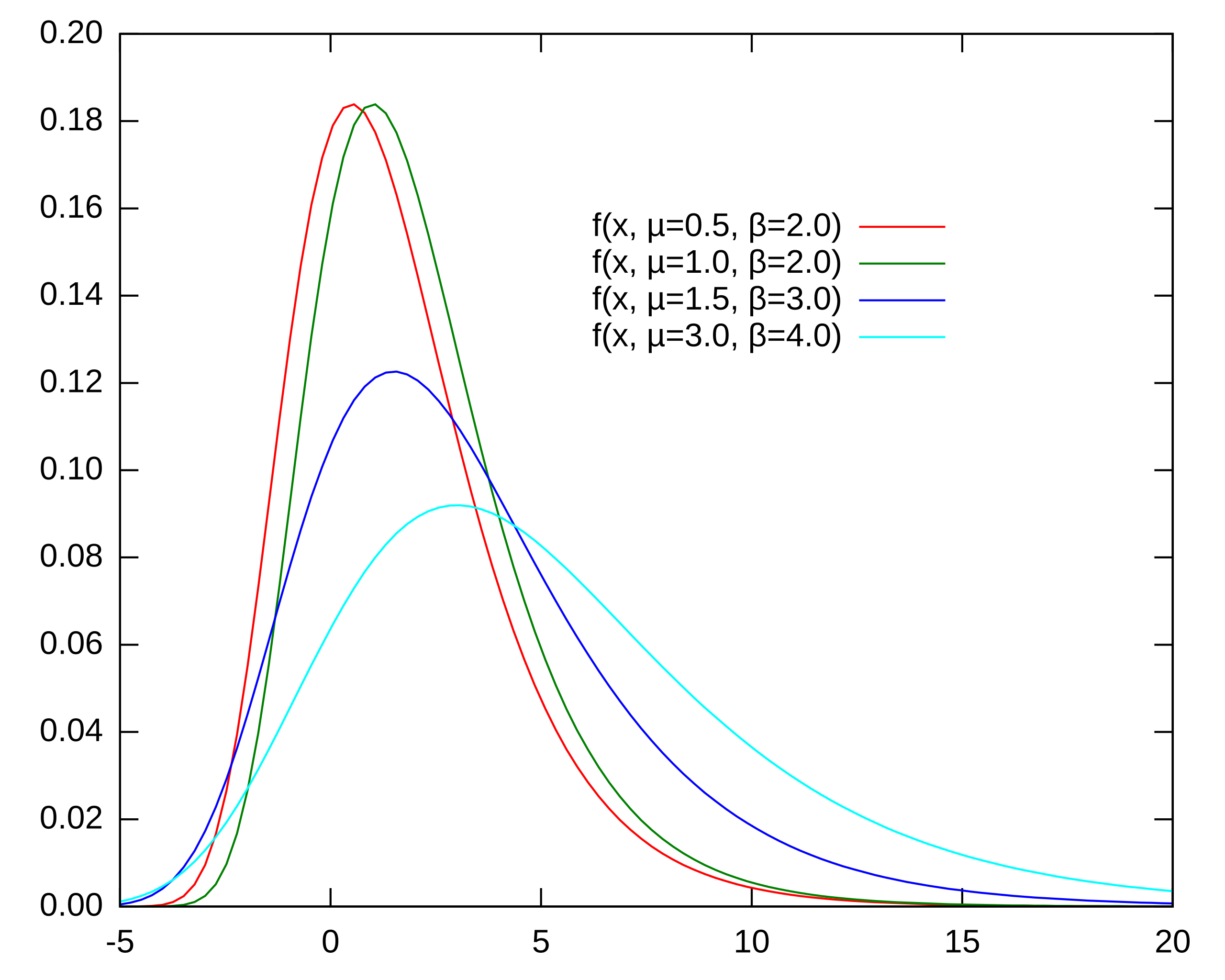
This distribution also known as Gumbel distribution was developed to study the maxima of independent random variables, wit applications to max level of a river, or maximum strength of an earthquake.

Extreme value theory = theory of distributions of extrema of random variables showed that there are three limiting distributions of maxima, thus “type I”.

Max stability

EV1 is a max-stable distribution \(\iff\) for any finite collection of random variables \(X_1, \ldots, X_n\) with the same distribution as \(X\), the random variable \(M_n = \max(X_1, \ldots, X_n)\) has the same distribution as \(X\) (up to location and scale).

What is an example of sum-stable (or simply stable) distribution?

Let \(\{X_i\}_{i=1,\dots,n}\) be a collection of independent random variables with the same CDF \(F(x)\). What is the CDF of the \(\max_i\{X_i\}\)?

Denote this CDF as \(F^{\mathrm{max}}_n(x)\).

\[\begin{split} \begin{array}{l} F^{\mathrm{max}}_n(x) \equiv Pr\{\max_i\{X_i\} \leqslant x\} = \\ = Pr\{X_1 \leqslant x, \ldots, X_n \leqslant x\} = \\ = \prod_{i=1}^n Pr\{X_i \leqslant x\} = \left[F(x)\right]^n \end{array} \end{split}\]

Therefore for EV1 distribution

\[\begin{split} \begin{array}{l} F^{\mathrm{max}}_n(x) = \left[F(x)\right]^n =\\ = [\exp\left(-\exp(-\tfrac{x-\mu}{\sigma})\right)]^n =\\ = \exp\left(-n\exp(-\tfrac{x-\mu}{\sigma})\right) =\\ = \exp\left(-\exp \ln \big[ n \exp(-\tfrac{x-\mu}{\sigma})\big]\right) =\\ = \exp\left(-\exp \ln \big[ n \exp(-\tfrac{x}{\sigma}) \exp(\tfrac{\mu}{\sigma})\big]\right) =\\ = \exp\left(-\exp \left[ -\tfrac{x}{\sigma} + \ln n + \ln \exp(\tfrac{\mu}{\sigma})\right]\right) =\\ = \exp\left(-\exp \left[ -\frac{x-\sigma [\ln n +\tfrac{\mu}{\sigma}]}{\sigma} \right]\right) = \\ = \exp\left(-\exp \left[ -\frac{x-\mu - \sigma \ln n}{\sigma} \right]\right) \end{array} \end{split}\]

Observe that the resulting CDF is EV1 with the same scale parameter \(\sigma\) and new location parameter equal \(\mu + \sigma \ln n\).

Imagine now that the \(n\) initial random variables have EV1 distribution with identical scale but different location parameters \(\mu_i\), with CDF denoted \(F_i(x)\). The completely analogous derivations gives

\[\begin{split} \begin{array}{l} F^{\mathrm{max}}_n(x) = \Pi_{i=1}^n F_i(x) =\\ = \Pi_{i=1}^n \exp\left(-\exp(-\tfrac{x-\mu_i}{\sigma})\right) =\\ = \exp\left(- \sum_{i=1}^n \exp(-\tfrac{x-\mu_i}{\sigma})\right) =\\ = \exp\left(-\exp \ln \big[ \sum_{i=1}^n \exp(-\tfrac{x-\mu_i}{\sigma})\big]\right) =\\ = \exp\left(-\exp \ln \big[ \exp(-\tfrac{x}{\sigma}) \sum_{i=1}^n \exp \tfrac{\mu_i}{\sigma}\big]\right) =\\ = \exp\left(-\exp \left[ -\tfrac{x}{\sigma} + \ln \sum_{i=1}^n \exp \tfrac{\mu_i}{\sigma}\right]\right) =\\ = \exp\left(-\exp \left[ -\frac{x-{\color{red} \sigma \ln \sum_{i=1}^n \exp \tfrac{\mu_i}{\sigma}}}{\sigma} \right]\right) \end{array} \end{split}\]

Again, the resulting CDF is EV1 with the same scale parameter \(\sigma\) and new location parameter equal

\[ \mu^{\mathrm{max}}_n = \sigma \ln \sum_{i=1}^n \exp \tfrac{\mu_i}{\sigma} \]

The expression for \(\mu^{\mathrm{max}}_n\) is typically referred to as logsum formula

Thus, we obtain that the maximum of EV1 random variables with varying location parameters is also an EV1 random variable, and its expectation is given by

\[ X_i \sim \mathrm{EV1}(\mu_i, \sigma), i=1,\dots,n \iff \mathbb{E} \max_{i=1,\dots,n} \{X_i\} = \sigma \ln \sum_{i=1}^n \exp \tfrac{\mu_i}{\sigma} + \sigma \gamma \]

Derivation of multinomial logit choice probabilities

Marschak [1960] showed that Luce’s structure of the choice probabilities obtains with RUM specification where the unobserved component \(\epsilon(d)\) are i.i.d. over alternatives \(d\), and have EV1 distribution

\[d^*(x,\epsilon)= \arg\max_{d \in D(x)} [u(x,d)+\epsilon(d)], \; \epsilon(d) \sim \mathrm{ EV1, i.i.d.}\]

Key assumption: independence across alternatives

Without loss of generality we can assume that \(\mu=0\) and \(\sigma=1\).

Indeed, consider EV1\((\mu,\sigma)\) random variable \(X\), and its counterpart \(\check{X}\) with distribution EV1\((0,1)\). We have

\[ Pr\{X < \sigma x+\mu\} = F(\sigma x+\mu) = \exp\big(-\exp(-x)\big) = Pr\{\check{X} < x\}, \]

and thus \(\check{X} = \frac{X-\mu}{\sigma}\).

Recall that constants and the scale of the utility function does not affect the choice probabilities. Therefore the equivalent to the above choice problem can be written as

\[ d^*(x,\epsilon)= \arg\max_{d \in D(x)} \left[\frac{u(x,d)}{\sigma}+\frac{\epsilon(d)-\mu}{\sigma}\right], \]

where the random term has standard extreme value distribution EV1(0,1)

Standard normalization assumption \(\mu=0\) and \(\sigma=1\)

Let us derive choice probabilities under EV1(0,1) i.i.d. distribution for \(\epsilon(d)\). For clarity, we temporarily denote \(\epsilon(d)\) as \(\xi \sim \mathrm{EV1}(0,1)\) and \(D'(x) = D(x) \setminus \{d\}\).

\[\begin{split} \begin{array}{l} P(d|x)= \hbox{Prob}\left\{d^*(x,\epsilon)=d|x\right\} =\\ = {\displaystyle \int_{-\infty}^{+\infty}} \hbox{Prob}\left\{ \max_{d' \in D'(x)} \big[u(d',x)+\epsilon(d')\big] \leqslant u(d,x)+\xi\right\} dF(\xi) = \\ = {\displaystyle \int_{-\infty}^{+\infty}} \hbox{Prob}\left\{ \max_{d' \in D'(x)} \big[\epsilon(d')+u(d',x)-u(d,x)\big] \leqslant \xi\right\} dF(\xi) = \\ = {\displaystyle \int_{-\infty}^{+\infty}} \exp\left( -\exp \Big[ - \xi + \ln \sum_{d' \in D'(x)} \exp \big(u(d',x)-u(d,x)\big)\Big] \right) \exp\big(-\xi-\exp(-\xi)\big) d\xi = \\ = {\displaystyle \int_{-\infty}^{+\infty}} \exp\left( -\exp \Big[ - \xi + \ln \sum_{d' \in D'(x)} \exp \big(u(d',x)-u(d,x)\big)\Big] -\exp(-\xi) \right) \exp(-\xi) d\xi = \\ = {\displaystyle \int_{-\infty}^{+\infty}} \exp\left( -\exp(-\xi) \Big[ \sum_{d' \in D'(x)} \exp \big(u(d',x)-u(d,x)\big)+1\Big] \right) \exp(-\xi) d\xi = \\ = {\displaystyle \int_{-\infty}^{+\infty}} \exp\left( -\exp(-\xi) \sum_{d' \in D(x)} \exp \big(u(d',x)-u(d,x)\big) \right) \exp(-\xi) d\xi = \\ = {\displaystyle \int_{-\infty}^{0}} \exp\left( t \sum_{d' \in D(x)} \exp \big(u(d',x)-u(d,x)\big) \right) dt = \\ = \left.\frac {\exp\left( t \sum_{d' \in D(x)} \exp \big(u(d',x)-u(d,x)\big) \right)} {\sum_{d' \in D(x)} \exp \big(u(d',x)-u(d,x)\big)} \right|_{-\infty}^{0} = \frac {1} {\sum_{d' \in D(x)} \exp \big(u(d',x)-u(d,x)\big)} = \frac {\exp u(d,x) } {\sum_{d' \in D(x)} \exp u(d',x)} \end{array} \end{split}\]

The logic under the derivation above is the following:

• fix the random component \(\xi = \epsilon(d)\) and integrate over its distribution on the outer loop

• probability that \(d\) is the maximizer of the random utility is the same as \(u(d,x)+ \xi\) being not less than the maximum of the rest of the utilities

• maximum of the random utilities is given by the maximum of the shifted EV1 random variables, distribution is known due to max-stability, with location parameter given by logsum formula

• then careful algebra with negative exponents

• variable substitution \(t = -\exp(-\xi)\) \(\implies dt = \exp(-\xi)d\xi\)

More generally, the following theorem holds for RUM models not necessarily with the EV1 error terms:

Williams-Daly-Zachary Theorem

Given a RUM model with absolutely continuous distribution of random terms \(\epsilon\)

\[d^*(x,\epsilon)= \arg\max_{d \in D(x)} [u(x,d)+\epsilon(d)],\]

the choice probabilities \(P(d|x)\) are given by

\[ P(d|x) = \frac{\partial}{\partial u(d,x)} \mathbb{E}\left\{\max_{d' \in D(x)} \big[ u(d',x) +\epsilon(d') \big]\Big|x\right\} \]

The value \(\mathbb{E}\left\{\max_{d' \in D(x)} \big[ u(d',x) +\epsilon(d') \big]\Big|x\right\}\) is known as McFadden’s social surplus function [McFadden, 1981].

Intuition for the proof:

\[\begin{split} \begin{array}{l} \frac{\partial}{\partial u(d,x)} \mathbb{E}\left\{\max_{d' \in D(x)} \big[ u(d',x) +\epsilon(d') \big]\Big|x\right\} =\\ = \frac{\partial}{\partial u(d,x)} {\displaystyle \int_\epsilon} \max_{d' \in D(x)} \big[ u(d',x) +\epsilon(d') \big] q(\epsilon|x) d\epsilon =\\ = {\displaystyle \int_\epsilon} \frac{\partial}{\partial u(d,x)} \max_{d' \in D(x)} \big[ u(d',x) +\epsilon(d') \big] q(\epsilon|x) d\epsilon =\\ = {\displaystyle \int_\epsilon} I\left\{ d^*(x,\epsilon)=d\right\}q(\epsilon|x) d\epsilon =P(d|x) \end{array} \end{split}\]

In case of EV1(0,1) it is easy to verify

\[\begin{split} \begin{array}{l} \frac{\partial}{\partial u(d,x)} \mathbb{E}\left\{\max_{d' \in D(x)} \big[ u(d',x) +\epsilon(d') \big]\Big|x\right\} =\\ = \frac{\partial}{\partial u(d,x)} \left[ \ln \sum_{d'\in D(x)} \exp u(d',x) + \gamma \right] =\\ = \frac{\exp u(d,x)}{\sum_{d'\in D(x)} \exp u(d',x)} \end{array} \end{split}\]

This is the alternative way to obtain the familiar multinomial logit choice probability

\[ P(d|x) = \frac{\exp u(d,x)}{\sum_{d'\in D(x)} \exp u(d',x)} \]

Advantages of logit

1. Choice probabilities are necessarily bounded between 0 and 1.

2. Choice probabilistic necessarily sum up to 1.

The scale parameter

In models with non-linear utility specification the scale parameter \(\sigma\) may be useful \(\rightarrow\) we may not want to impose normalization \(\sigma = 1\)

It is not too hard to repeat the above derivations with \(\sigma\) present in all expressions, and obtain

\[ P(d|x) = \frac{\exp \big(u(d,x)/\sigma\big)}{\sum_{d'\in D(x)} \exp \big(u(d',x)/\sigma\big)} \]

As \(\sigma \to \infty\) each exponent in the expression approaches zero, and \(P(d|x) \to 1/|D(x)|\), that is choice probabilities approach uniform distribution.

Conversely, as \(\sigma \to 0\) the choice probabilities become increasingly sensitive to differences in utility, and \(P(d|x)\) approaches a deterministic choice \(P(d|x) = I \big\{u(d,x) > u(d',x), \forall d' \in D(x)\setminus \{d\}\big\}\), that is the distribution collapses to a point mass at the alternative with highest utility.

Disadvantages of IIA and generalizations

Luce made IIA the foundation of the probabilistic choice model, but it is not necessarily a good model. Sometimes choice behavior exhibits patterns of substitution that are not captured by IIA.

Example: red - blue bus paradox

• Suppose a person can commute to work by “blue bus” \(b\) or car \(c\) and \(u(b,x) = u(c,x)\)

• Logit with IIA \(\implies\) \(P(b|x) = P(c|x) = 1/2\)

• Now suppose we do an experiment introducing a third artificial alternative “red bus” \(r\) which is the same as “blue” except the color, and thus \(u(r,x) = u(b,x) = u(c,x)\).

• Logit with IIA now predicts \(P(b|x) = P(r|x) = P(c|x) = 1/3\)

• However, more reasonable prediction would be \(P(b|x) = P(r|x) = 1/4\) and \(P(c|x) = 1/2\)

The paradox in the blue-red bus example is due to independence of the error terms \(\epsilon\) across alternatives, which is clearly brocken here as blue and red busses only differ in color \(\implies\) their unobserved attributes captured by \(\epsilon\) are likely correlated

Remedies

In the cases when IIA is not desirable we need an alternative model of choice. Typical options:

• Probit model

  • Assumes a joint normal distribution of error terms

  • Flexibility of substitution patterns due to many parameters in the covariance matrix

  • Requires multidimensional integration with no closed form

• GEV model

  • Generalization of the logit model

  • Relaxes the substitution pattern restrictions

  • Maintains the analytical closed form expressions for choice probabilities and social surplus function

• Mixed logit model

  • Integrates choice probabilities over randomly distributed components, for example allowing taste variation across decision makers

  • Allows for rich substitution patterns between alternatives

  • Can approximate any RUM choice problem

• Dynamic model

  • Relaxes IIA due to the continuation values of alternatives

See later chapters in 📖 Train [2009] “Discrete Choice Methods with Simulation” for further details

Random coefficients mixed logit

Assume that the utility function in a random utility model is given by \(u(d,x) = x_d \tilde{\beta}\) where \(x_d\) is a vector of alternative attributes and \(\tilde{\beta}\) is a vector of random coefficients distributed Normally with means \(\mu\) and covariance matrix \(\Sigma\):

\[ u(d,x_d) = x_d \tilde{\beta}, \; \tilde\beta \sim N(\mu,\Sigma) \]

Then the RUM can be expressed as:

\[ u(d,x_d) + \epsilon(d) = x_d \mu + x_d (\tilde{\beta}-\mu), \epsilon(d)=x_d (\tilde{\beta}-\mu) \sim N(0,x_d\Sigma x_d') \]

Now as two alternatives become close, \(x_d \approx x_{d'}\), their corresponding errors \(\epsilon(d)\) and \(\epsilon(d')\) become perfectly correlated

\[ \mathrm{var}(\epsilon(d)-\epsilon(d')) = \mathrm{var}((x_d-x_{d'}) (\tilde{\beta}-\mu)) = (x_d - x_{d'}) \Sigma (x_d - x_{d'})' \approx 0 \implies \epsilon(d) \approx \epsilon(d') + \mathrm{const} \]

Generalized extreme value (GEV)

The distribution is given by the following CDF

\[ G(\epsilon_1,\dots,\epsilon_K)= \exp \Big( -\mathcal{H}\big( \exp(-\epsilon_1+v_1),\dots,\exp(-\epsilon_K+v_K) \big) \Big), \]

where \(v_1,\dots,v_K\) are location parameters, and the GEV generating function \(\mathcal{H}: \mathbb{R}_{+}^K \to \mathbb{R}_{+}\) satisfies the conditions listed in [McFadden, 1981]:

• \(\mathcal{H}(x) \geqslant 0\), \(\forall x \in \mathbb{R}_{+}^K\)

• \(\mathcal{H}\) homogenous of degree \(\mu\geqslant 0\), i.e. \(\mathcal{H}(\lambda x) = \lambda^\mu \mathcal{H}(x)\) for all \(\lambda>0\)

• \(\mathcal{H}\) is differentiable with mixed partial derivatives for \(j=1,\dots,K\) satisfying

\[ (-1)^j\frac{\partial^j \mathcal{H}}{\partial x_1 \dots \partial x_K} \leqslant 0 \]

McFadden [1981] shows that if vector \((\epsilon_1,\dots,\epsilon_K)\) has GEV distribution with generating functon \(\mathcal{H}\), then it holds:

1. Each \(\epsilon_j\) for \(j \in 1,\dots,K\) has EV1 distribution with common variance \(\pi^2/6\mu^2\) and means \((\log \mathcal{H}(1_j)+\gamma)/\mu\), where \(1_j\) is a vector of zeros with a one in the \(j\)-th position;

2. Max-stability: \(\max_{i=1,\dots,K} \{\epsilon_i\}\) has an EV1 distribution with the same variance and mean \(\big[\log \mathcal{H}(\exp(v_1),\dots,\exp(v_K))+\gamma\big]/\mu\);

3. Denoting \(\mathcal{H}_i(\cdot)\) the partial derivative of \(\mathcal{H}\) with respect to the \(i\)-th argument, the choice probabilities are given by

\[ P(d|v) = \frac{\exp(v_d) \mathcal{H}_d(\exp(v_1),\dots,\exp(v_K)) }{\mu \mathcal{H}(\exp(v_1),\dots,\exp(v_K))} \]

Flexibility of the \(\mathcal{H}\) function allows for a wide range of substitution patterns between alternatives.

\[ \mathcal{H}(w) = \sum_{i=1}^{K} w_i \quad \implies \quad \text{multinomial logit} \]

\[ \mathcal{H}(w) = \sum_{i=1}^{M} \left( \sum_{j \in I_i} w_i^\tau \right)^{\tfrac{1}{\tau}}, \cup_i I_i = \{1,\dots,K\}, I_{i_1} \cap I_{i_2} = \emptyset \; \implies \; \text{nested logit} \]

Note that scale parameters must form a non-increasing sequence when moving to inner nests to satisfy the conditions on \(\mathcal{H}\)

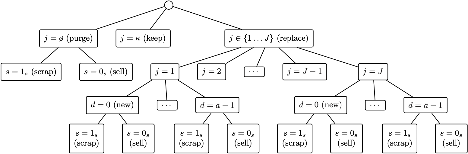
Example

Choice tree from [Gillingham, Iskhakov, Munk-Nielsen, Rust, and Schjerning, 2022] showing the nested alternatives conditioning on having a car

Smoothing of kinks and discontinuities

Many rules and policies are represented in economic models with kinky or even discontunous functions:

• progressive tax rules with kinks at the bracket thresholds

• social support programs, pension rules

• upper envelope of families of functions (discrete-continuous choice, see [Iskhakov, Jørgensen, Rust, and Schjerning, 2017])

• upper envelope of likelihood correspondence in games with multiple equilibria

Logistic models have a great use as numerical smoothing devices in many of such situations

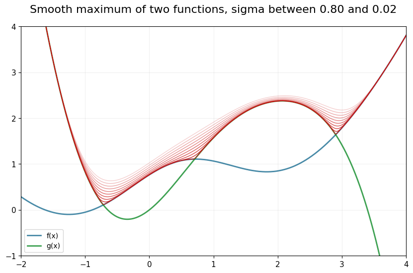
Smoothing kinks

Consider two functions \(f(x)\) and \(g(x)\) defined over some range \(X\). Imagine we are interested in \(h(x) = \max\big(f(x), g(x)\big)\), which has kinks in general case at the point where it holds \(f(x)=g(x)\).

The following function is a smooth version of \(h(x)\)

\[ \tilde{h}(x) = \sigma\log\big(\exp(f(x)/\sigma) + \exp(g(x)/\sigma)\big) \to h(x) \;\text{ as }\;\sigma \to 0 \]

Show code cell source

Hide code cell source

import matplotlib.pyplot as plt
import numpy as np
x = np.linspace(-2, 4, 1000)
f1 = 2 * np.exp(-0.5 * (x - 0.5)**2) + 0.3 * x**2 - 1
f2 = -0.4 * x**3 + 1.2 * x**2 + 0.5 * x + 0.5 + 0.3 * np.sin(2*x)-0.5
f3 = lambda sigma: sigma * np.log(np.exp(f1/sigma) + np.exp(f2/sigma))
# Plot the functions
fig, ax = plt.subplots(figsize=(10, 6), dpi=100)
ax.plot(x, f1, linewidth=2.0, color="#1A6D91", label='f(x)', alpha=0.8)
ax.plot(x, f2, linewidth=2.0, color="#0E8A27", label='g(x)', alpha=0.8)
ax.legend(frameon=True, loc='lower left')
s1,s2=0.02,0.8
for sigma in np.linspace(s1, s2, 10):
  ax.plot(x, f3(sigma), linewidth=1.0, color="#CB1515", label=f'logsum(f1,f2,simga={sigma:0.3f})', alpha=1 - sigma)
ax.set_title(f'Smooth maximum of two functions, sigma between {s2:0.2f} and {s1:0.2f}', fontsize=16, pad=20)
ax.grid(True, alpha=0.3, linestyle='-', linewidth=0.5)
ax.tick_params(axis='both', which='major', labelsize=11)
ax.set_xticks(np.arange(-2, 5, 1))
ax.set_yticks(np.arange(-1, 5, 1))
ax.set_xlim(-2, 4)
ax.set_ylim(-1, 4)
plt.show()

What is the biggest discrepancy between \(h(x)\) and \(\tilde h(x)\)?

\[ \tilde h(x) - h(x) \to \max(x) \]

Equivalently because \(\exp(x/\sigma)\) is a monotone increasing transformation when \(\sigma>0\) we could solve

\[ \exp\frac{\tilde h(x) - h(x)}{\sigma} = \frac{\exp(f(x)/\sigma) + \exp(g(x)/\sigma)} {\exp(\max\big[f(x),g(x)\big]/\sigma)} \to \max(x) \]

We can see that if \(f(x)\geqslant g(x)\) the expression collapses to \(1 + \exp\frac{g(x) - f(x)}{\sigma} \leqslant 2\). Conversely, if \(f(x)\leqslant g(x)\) the expression becomes \(\exp\frac{f(x) - g(x)}{\sigma} +1 \leqslant 2\). The maximum of 2 is attained when \(f(x) = g(x)\)!

We conclude that

\[ \max \{ \tilde h(x) - h(x) \} = \sigma \ln2 \]

Therefore, the discrepancy error is easily controlled by choosing an appropriate value for \(\sigma\).

This technique can be generalized to more functions and higher dimension.

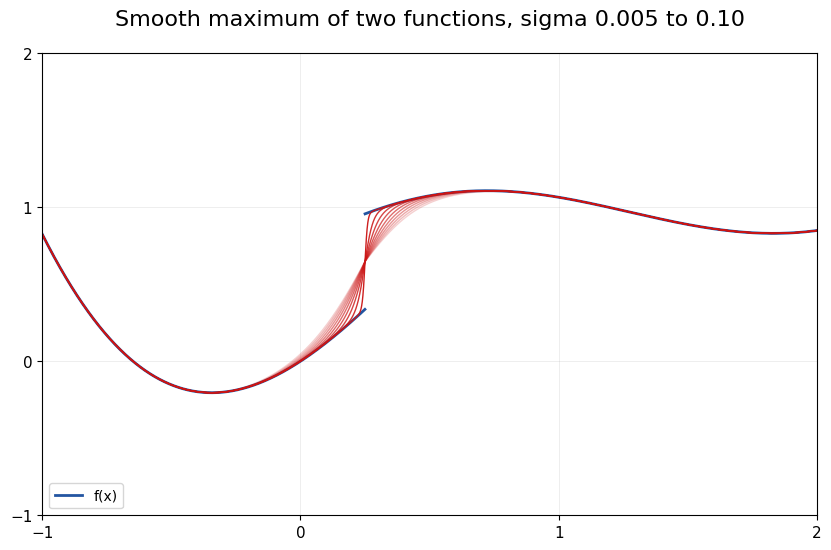
Smoothing discontinuities

Now consider a function \(f(x)\) which is smooth except for the point \(x_0\) where it has a discontinuous jump, without loss of generality jump up.

The smoothing device in this case is a logistic choice probability rather than logsum:

\[ \tilde f(x) = f(x) + \bar{f} \left[ \frac{\exp\tfrac{x-x_0}{\sigma}}{1 + \exp\tfrac{x-x_0}{\sigma}} - I\{x>x_0\} \right] \to f(x) \;\text{ as }\;\sigma \to 0, \]

where \(\bar{f} = \lim_{x\to x_0^+} f(x) - \lim_{x\to x_0^-} f(x)\) is the size of the jump.

Unlike in the previous case, convergence here is pointwise rather than uniform because the smoothed \(\tilde f(x)\) will always be off from the true \(f(x)\) by \(\bar{f}/2\) at the jump point, and this discrepancy does not disappear as \(\sigma \to 0\).

Show code cell source

Hide code cell source

import matplotlib.pyplot as plt
import numpy as np
x0=0.25
x = np.linspace(-1, 2, 10000)
f1 = lambda x: -0.4 * x**3 + 1.2 * x**2 + 0.5 * x + 0.5 + 0.3 * np.sin(2*x)-0.5
f2 = lambda x: 2 * np.exp(-0.5 * (x - 0.5)**2) + 0.3 * x**2 - 1
f = lambda x: (x<x0)*f1(x) + (x>x0)*f2(x)
fd = f(x)
ix = np.max(np.where(x <= x0))
gap = f2(x[ix])-f1(x[ix])
fd[ix]=np.nan # to show discontinuity
g = lambda x,sigma: fd + gap*(1/(1+np.exp(-(x-x0)/sigma))-(x>x0))
# Plot the functions
fig, ax = plt.subplots(figsize=(10, 6), dpi=100)
ax.plot(x, fd, linewidth=2.0, color="#2355A1", label='f(x)', alpha=1.)
ax.legend(frameon=True, loc='lower left')
s1,s2=0.005,0.1
for sigma in np.linspace(s1, s2, 10):
  ax.plot(x, g(x,sigma), linewidth=1.0, color="#CB1515", label=f'logsum(f1,f2,simga={sigma:0.3f})', alpha=(1 - 8*sigma))
ax.set_title(f'Smooth maximum of two functions, sigma {s1:0.3f} to {s2:0.2f}', fontsize=16, pad=20)
ax.grid(True, alpha=0.3, linestyle='-', linewidth=0.5)
ax.tick_params(axis='both', which='major', labelsize=11)
ax.set_xticks(np.arange(-2, 5, 1))
ax.set_yticks(np.arange(-1, 5, 1))
ax.set_xlim(-1, 2)
ax.set_ylim(-1, 2)
plt.show()

De-maxing when computing logit probabilities and logsums

One last point before the practical work.

Do you expect the following code to run without errors

a = 2.
for i in range(20):
  print(f"{i} exp({a})={np.exp(a)}")
  a **= 1.25

Exponentiation on a computer is potentially dangerous!

This is due to overfolow: when the number gets too big, it can no longer be represented in the finite space of bits and an error occurs

Thankfully, we have a very good way to make logit choice probabilities and logsums much more numerically stable:

\[ \frac{\exp(x_i)}{\sum_{j=1}^{K} \exp(x_j)} = \frac{\exp(x_i-M)}{\sum_{j=1}^{K} \exp(x_j-M)} \]

If we let \(M = \max_j(x_j)\) then we are only exponentiating negative numbers, and even though there is a risk of underflow error, we would be replacing a very small number with exactly zero which is ok \(\rightarrow\) numerical stability

\[ \log \left( \sum_{j=1}^{K} \exp(x_j) \right) = \log \left( \sum_{j=1}^{K} \exp(x_j - M) \right) + M \]

Analogously, it is possible to avoid computing exponents of large numbers.

Always remember to DEMAX the values going into computation of logit probabilities and logsums!

References and Additional Resources

• 📖 Train [2009] “Discrete Choice Methods with Simulation” Online book
  chapter 1
chapter 2
chapter 3
chapter 4
  

• 📖 Math note by Victor Aguirregabiria on logit, nested logit and ordered logit models pdf