📖 Dynamic Programming

⏱ | words

References

What is dynamic programming?

“DP is recursive method for solving sequential decision problems”

📖 Rust 2006, New Palgrave Dictionary of Economics

In computer science the meaning of the term is broader: DP is a general algorithm design technique for solving problems with overlapping sub-problems.

Dynamic programming in economics

DP provides a framework to study decision making over time and under uncertainty and can accommodate learning, strategic interactions between agents (game theory) and market interactions (equilibrium theory)

Many important problems and economic models are analyzed and solved using dynamic programming:

• Dynamic models of labor supply

• Job search

• Human capital accumulation

• Health process, insurance and long term care

• Consumption/savings choices

• Durable consumption

• Growth models

• Heterogeneous agents models

• Overlapping generation models

Dynamic discrete choice (DDC)

Extend the discrete choice framework to repeated discrete choice over time

• Given state \(s_t \in S\) an agent takes a decision \(d_t \in D(s)\) that determines current utility \(u_t(s_t,d_t)\) as well as the future states of the world.

• The agent forms (subjective) beliefs about the uncertain next period’s state \(s_{t+1}\) that evolve according to a Markov transition probability \(p(s_{t+1}|s_t, d_t)\).

• The agent’s problem is to choose a optimal decision rule \(\mathbf{\delta} = \{\delta_0,...,\delta_T\}\), where \(d_t=\delta_t(s_t)\), that solves

\[ \max_{\mathbf{\delta}= \{\delta_0..... \delta_{T}\}} \mathbb{E}{_{\mathbf{\delta}}} \big[ \sum_{t=0}^T \beta^t u_t(s_t,d_t) | s_0=s \big] \]

where \(\mathbb{E}_{\delta}\) denotes expectation with respect to the controlled stochastic process \(\{s_t,d_t\}\) induced by the decision rule \(\delta\).

• The difficulty is that we are looking for a set of functions \(\mathbf{\delta} = \{\delta_0,...,\delta_T\}\), not just for a set of numbers \(\mathbf{d} = \{d_0,...,d_T\}\)

• DP simplifies the DDC problem, allowing us to find \(\mathbf{\delta} = \{\delta_0,...,\delta_T\}\) using a recursive procedure.

Bellman’s Principle of Optimality

An optimal policy has a property that whatever the initial state and initial decision are, the remaining decisions must constitute an optimal policy with regard to the state resulting from the first decision.

📖 Bellman, 1957 “Dynamic Programming”

Breaking the problem into sequence of small problems

• Thus, the sequential decision problem is broken into initial decision problem and the future decisions problem

• The solution can be computed through backward induction, i.e. solving a sequential decision problem from the later periods

• Embodiment of the recursive way of modeling sequential decisions is Bellman equation

Bellman equation

Definition

Bellman equation is the complete recursive description of the dynamic optimization problem in discrete time:

\[V(\text{state}) = \max_{\text{decisions}} \big[ U(\text{state},\text{decision}) + \beta \mathbb{E}\big\{ V(\text{next state}) \big| \text{state},\text{decision} \big\} \big]\]

• State variables — vector of variables that describe all relevant information about the modeled decision process, \(x_t\)

• Decision variables — vector of variables describing the choices, \(d_t\)

• Instantaneous payoff — utility function, \(u(x_t,d_t)\), with time separable discounted utility

• (next state) is the stochastic next period state resulting from current state and decision

• expectation \(\mathbb{E}\{\cdot\}\) is taken over the distribution of the next period state conditional on current state and decision

• Motion rules — agent’s beliefs of how state variable evolve through time, conditional on choices, \(x_{t+1} \sim F(x_t,d_t)\)

• \(\beta\) is a discount factor to measure future rewards in terms of current ones

Solution is given by:

• Value function — maximum attainable utility \(V(x_t)\)

• Policy function — mapping from state space to action space that returns the optimal choice, \(d^{\star}(x_t)\)

The optimal choices are revealed along the solution of the Bellman equation as decisions which solve the maximization problem in the right hand side (\(\arg\max\) of the maximization in the Bellman equation)

Classification of DP models

• Discrete or continuous time?

• Finite or infinite horizon?

• Choice space (discrete, continuous, mixed)?

• State space (finite, discretized)?

• Stochastic or deterministic evolution of states?

Whether choice is part of the problem at all

• Computer science uses DP to solve problems without explicit decisions, but breaking big problems into a series of small ones lecture 27 in CompEcon course

• Examples of sequential discrete/discretized choice

  • deal or no deal problem lecture 27 in CompEcon course

  • inventory management model (see below)

  • Rust model of bus engine replacement lecture 28, 29 in CompEcon course

  • cake eating problem lecture 30, 32 in CompEcon course

  • consumption-savings problem lecture 35 in CompEcon course

Whether choice space is discrete, continuous, mixed discrete-continuous or discretized

1. Problems with discrete choice

   • deal or no deal problem, inventory management model lecture 27 in CompEcon course

   • Rust model of bus engine replacement lectures 28, 29 in CompEcon course

2. Problems with continuous choice

   • discretized: cake eating problem lecture 30 in CompEcon course , consumption-savings models lecture 35 in CompEcon course

   • treated as continuous: coming up next

   • require interpolating of value function in Bellman equation

3. Problems with discrete and continuous choice

   • much more complicated: kinks in value functions, discontinuous policy function

   • require global optimization in Bellman equation which is not easy

   • one way out is to discretize choices at the cost of reduced accuracy

   • see our paper Iskhakov et al. [2017] for how to smooth the kinks

What about state space?

• When choice is discrete, typically state space is also finite

• Even when state variables are continuous, by discretization it is converted to discrete

1. This is true in general when using numerical solvers: state space is discretized within some reasonable bounds

   • choice of upper bounds, number and placement of grid points influence the (accuracy of the) solution

2. Another approach to represent state space is to project value and/or policy function onto space of orthogonal polynomials (Chebyshev polynomials in particular)

   • only works well when value function is sufficiently smooth

Whether time is continuous or discrete

1. Discrete time

   • time periods \(t\), \(t+1\)

   • dynamics given by difference equations

2. Continuous time

   • all entities in the model are functions of time

   • dynamics given by differential equation

   • so, math is very different

   • continuous time for cleaner theoretical models, sometimes also solved numerically

   • not part of this course

Whether horizon is finite or infinite

1. Finite horizon

   • there is terminal period \(T\)

   • special form of Bellman equation in period \(T\)

   • in other words, as if \(V(\text{at } T +1 ) = \mathbb{0}\)

   • value function and policy function are time dependent

   • solved by backwards induction with \(T\) number of steps

\[V(\text{state}) = \max_{\text{decisions}} \big[ U(\text{state},\text{decision}) \big] \text{ at terminal period } T\]

2. Infinite horizon

   • time subscripts are dropped, primes for next period values instead

   • solution is given by fixed point of the Bellman operator

   • have to actually solve a functional equation

Most problems can be specified and solved in both finite or infinite horizon

Whether model includes stochastic processes

1. Deterministic models

   • No random elements, all motion rules deterministic

   • No need for expectation operator in Bellman equation

\[V(\text{state}) = \max_{\text{decisions}} \big[ U(\text{state},\text{decision}) + \beta \cdot V(\text{next state}) \big]\]

2. Stochastic models with idiosyncratic shocks

   • expectation does not have to be conditioned on current period shocks

   • solving the fixed point in expected value function space is beneficial

3. General form stochastic models

   • expectation in Bellman equation has to be computed with quadrature or Monte Carlo integration

Example: Inventory management model

Consider the following problem in discrete time and finite horizon \(t=0,\dots,T\)

The notation is:

• \(x_t\ge 0\) is inventory at period \(t\) measured in discrete units

• \(d_t\ge 0\) is potentially stochastic demand at period \(t\)

• \(q_t\ge 0\) is the order of new inventory

• \(p\) is the profit per one unit of (supplied) good

• \(c\) is the fixed cost of ordering any amount of new inventory

• \(r\) is the cost of storing one unit of good

The sales in period \(t\) are given by \(s_t = \min\{x_t,d_t\}\).

Inventory to be stored till next period is given by \(k_t = \max\{x_t-d_t,0\} + q_t = x_{t+1}\).

The profit in period \(t\) is given by

\[\begin{split} \begin{array}{rcl} \pi_t & = & p \cdot \text{sales}_t - r \cdot x_{t+1} - c \cdot (\text{order made in period }t) \\ & = & s_t p - k_t r - c \mathbb{1}\{q_t>0\} = \\ & = & p \min\{x_t,d_t\} - r \big[ \max\{x_t-d_t,0\} + q_t \big] - c \mathbb{1}\{q_t>0\} \end{array} \end{split}\]

Assuming all \(q_t \ge 0\), let \(\sigma = \{q_t\}_{t=1,\dots,T}\) denote a feasible inventory policy.

If \(d_t\) is stochastic the policy becomes a function of the period \(t\) inventory \(x_t\).

The expected profit maximizing problem is given by

\[{\max}_{\sigma} \mathbb{E}\Big[ \sum_{t=0}^{T} \beta^t \pi_t \Big],\]

where \(\beta\) is discount factor.

Bellman equation for the problem

Decisions: \(q_t\), how much new inventory to order

What is important for the inventory decision at time period \(t\)?

• instanteneous utility (profit) contains \(x_t\) and \(d_t\)

• timing / sequence of events:

  • (beginning of period)

  1. current inventory

  2. demand

  3. order (choice)

  4. stored inventory

  • (end of period)

So, both \(x_t\) and \(d_t\) are taken into account for the new order to be made, forming the state space.

\[\begin{split} \begin{array}{rcl} V(x_t,d_t) &=& \max_{q_t \ge 0} \Big\{ \pi_t + \beta \mathbb{E}\Big[ V\big(x_{t+1} , d_{t+1} \big) \Big| x_t,d_t,q_t \Big] \Big\} \\ &=& \max_{q_t \ge 0} \Big\{ s_t p - k_t r - c \mathbb{1}\{q_t>0\} + \beta \mathbb{E}\Big[ V\big( k_t, d_{t+1} \big) \Big] \Big\} \end{array} \end{split}\]

\[\begin{split} \begin{array}{rcl} s_t &=& \min\{x_t,d_t\} \\ k_t &=& \max\{x_t-d_t,0\} + q_t \end{array} \end{split}\]

The expectation in the Bellman equation is taken over the distribution of the next period demand \(d_{t+1}\), which we assume is independent of any other variables and across time (idiosyncratic), thus the conditioning on \((x_t,d_t,s_t)\) can be meaningfully dropped.

Expectation can be written as an integral over the distribution of demand \(F(d)\), and since inventory is discrete it’s natural to assume demand is as well.

The integral then transforms into a sum over the possible value of demand, weighted by their probabilities \(pr(d)\)

\[\begin{split} \begin{array}{rcl} V(x_t,d_t) &=& \max_{q_t \ge 0} \Big\{ s_t p - k_t r - c \mathbb{1}\{q_t>0\} + \beta \int V\big( k_t, d \big) \partial F(d) \Big\} \\ &=& \max_{q_t \ge 0} \Big\{ s_t p - k_t r - c \mathbb{1}\{q_t>0\} + \beta \sum_d V\big( k_t, d \big) pr(d) \Big\} \end{array} \end{split}\]

But let’s focus first on a deterministic case: let \(d\) be fixed and constant over time. How does the Bellman equation change?

In the deterministic case with fixed \(d\), it can be simply dropped from the state space, and the Bellman equation can be simplified to

\[ V(x_t) = \max_{q_t \ge 0} \big\{ p \min\{x_t,d\} - r \big[ \max\{x_t-d,0\} + q_t \big] - c \mathbb{1}\{q_t>0\} + \beta V\big( \max\{x_t-d,0\} + q_t \big) \big\} \]

How does this convert to the code?

import numpy as np
import matplotlib.pyplot as plt
%matplotlib inline
plt.rcParams['figure.figsize'] = [12, 8]

class inventory_model:
    '''Small class to hold model fundamentals and its solution'''

    def __init__(self,label='noname',
                 max_inventory=10,  # upper bound on the state space
                 c = 3.2,           # fixed cost of order
                 p = 2.5,           # profit per unit of good
                 r = 0.5,           # storage cost per unit of good
                 β = 0.95,          # discount factor
                 demand = 4         # fixed demand
                 ):
        '''Create model with default parameters'''
        self.label=label # label for the model instance
        self.c, self.p, self.r, self.β = c, p, r, β
        self.demand = demand
        # created dependent attributes (it would be better to have them updated when underlying parameters change)
        self.n = max_inventory+1    # number of inventory levels
        self.upper = max_inventory  # upper boundary on inventory
        self.x = np.arange(self.n)  # all possible values of inventory (state space)

    def __repr__(self):
        '''String representation of the model'''
        return 'Inventory model labeled "{}"\nParamters (c,p,r,β) = ({},{},{},{})\nDemand={}\nUpper bound on inventory {}' \
               .format (self.label,self.c,self.p,self.r,self.β,self.demand,self.upper)

    def sales(self,x,d):
        '''Sales in given period'''
        return np.minimum(x,d)

    def next_x(self,x,d,q):
        '''Inventory to be stored, becomes next period state'''
        return x - self.sales(x,d) + q

    def profit(self,x,d,q):
        '''Profit in given period'''
        return self.p * self.sales(x,d) - self.r * self.next_x(x,d,q) - self.c * (q>0)

model=inventory_model(label='test')
print(model)

q=np.zeros(model.n)
print('Current profits with zero orders\n',model.profit(model.x,model.demand,q))

Inventory model labeled "test"
Paramters (c,p,r,β) = (3.2,2.5,0.5,0.95)
Demand=4
Upper bound on inventory 10
Current profits with zero orders
 [ 0.   2.5  5.   7.5 10.   9.5  9.   8.5  8.   7.5  7. ]

# illustration of broadcasting in the inventory model
q=model.x[:,np.newaxis]  # column vector
print('Current inventory\n',model.x)
print('Current sales\n',model.sales(model.x,model.demand))
print('Current orders\n',q)
print('Next period inventory\n',model.next_x(model.x,model.demand,q))
print('Current profits\n',model.profit(model.x,model.demand,q))

Current inventory
 [ 0  1  2  3  4  5  6  7  8  9 10]
Current sales
 [0 1 2 3 4 4 4 4 4 4 4]
Current orders
 [[ 0]
 [ 1]
 [ 2]
 [ 3]
 [ 4]
 [ 5]
 [ 6]
 [ 7]
 [ 8]
 [ 9]
 [10]]
Next period inventory
 [[ 0  0  0  0  0  1  2  3  4  5  6]
 [ 1  1  1  1  1  2  3  4  5  6  7]
 [ 2  2  2  2  2  3  4  5  6  7  8]
 [ 3  3  3  3  3  4  5  6  7  8  9]
 [ 4  4  4  4  4  5  6  7  8  9 10]
 [ 5  5  5  5  5  6  7  8  9 10 11]
 [ 6  6  6  6  6  7  8  9 10 11 12]
 [ 7  7  7  7  7  8  9 10 11 12 13]
 [ 8  8  8  8  8  9 10 11 12 13 14]
 [ 9  9  9  9  9 10 11 12 13 14 15]
 [10 10 10 10 10 11 12 13 14 15 16]]
Current profits
 [[ 0.   2.5  5.   7.5 10.   9.5  9.   8.5  8.   7.5  7. ]
 [-3.7 -1.2  1.3  3.8  6.3  5.8  5.3  4.8  4.3  3.8  3.3]
 [-4.2 -1.7  0.8  3.3  5.8  5.3  4.8  4.3  3.8  3.3  2.8]
 [-4.7 -2.2  0.3  2.8  5.3  4.8  4.3  3.8  3.3  2.8  2.3]
 [-5.2 -2.7 -0.2  2.3  4.8  4.3  3.8  3.3  2.8  2.3  1.8]
 [-5.7 -3.2 -0.7  1.8  4.3  3.8  3.3  2.8  2.3  1.8  1.3]
 [-6.2 -3.7 -1.2  1.3  3.8  3.3  2.8  2.3  1.8  1.3  0.8]
 [-6.7 -4.2 -1.7  0.8  3.3  2.8  2.3  1.8  1.3  0.8  0.3]
 [-7.2 -4.7 -2.2  0.3  2.8  2.3  1.8  1.3  0.8  0.3 -0.2]
 [-7.7 -5.2 -2.7 -0.2  2.3  1.8  1.3  0.8  0.3 -0.2 -0.7]
 [-8.2 -5.7 -3.2 -0.7  1.8  1.3  0.8  0.3 -0.2 -0.7 -1.2]]

Backwards induction

Backwards induction algorithm is used to solve finite horizon models

Solver for the finite horizon dynamic programming problems

1. Start at t=T
1. Solve Bellman equation at t, record optimal choice  
1. Decrease t unless t=1, and return to previous step.  


As result, for all t=1,..,T have found the optimal choice (as a function of state)

First, we need to code up the Bellman equation

def bellman(m,v0):
    '''Bellman equation for inventory model
       Inputs: model object
               next period value function
    '''
    # create the grid of choices (same as x), column-vector
    q = m.x[:,np.newaxis]
    # compute current period profit (relying on numpy broadcasting to get the matrix with choices in rows)
    p = m.profit(m.x,m.demand,q)
    # indexes for next period value with extrapolation using last value
    i = np.minimum(m.next_x(m.x,m.demand,q),m.upper)
    # compute the Bellman maximand
    vm = p + m.β*v0[i]
    # find max and argmax
    v1 = np.amax(vm,axis=0)   # maximum in every column
    q1 = np.argmax(vm,axis=0) # arg-maximum in every column = order volume
    return v1, q1

v = np.zeros(model.n)
for i in range(3):
    v,q = bellman(model,v)
    print('Value =',v,'Policy =',q,sep='\n',end='\n\n')

Value =
[ 0.   2.5  5.   7.5 10.   9.5  9.   8.5  8.   7.5  7. ]
Policy =
[0 0 0 0 0 0 0 0 0 0 0]

Value =
[ 4.3    6.8    9.3   11.8   14.3   14.3   14.3   15.625 17.5   16.525
 15.55 ]
Policy =
[4 4 4 4 4 3 2 0 0 0 0]

Value =
[ 9.425 11.925 14.425 16.925 19.425 19.425 19.425 19.71  21.585 21.085
 20.585]
Policy =
[8 8 8 8 8 7 6 0 0 0 0]

def solver_backwards_induction(m,T=10,verbose=False):
    '''Backwards induction solver for the finite horizon case'''
    # solution is time dependent
    m.value  = np.zeros((m.n,T))
    m.policy = np.zeros((m.n,T))
    # main DP loop (from T to 1)
    for t in range(T,0,-1):
        if verbose:
            print('Time period %d\n'%t)
        j = t-1 # index of value and policy functions for period t
        if t==T:
            # terminal period: ordering zero is optimal
            m.value[:,j] = m.profit(m.x,m.demand,np.zeros(m.n))
            m.policy[:,j] = np.zeros(m.n)
        else:
            # all other periods
            m.value[:,j], m.policy[:,j] = bellman(m,m.value[:,j+1]) # next period to Bellman
        if verbose:
            print(m.value,'\n')
    # return model with updated value and policy functions
    return m

model = inventory_model(label='illustration')
model=solver_backwards_induction(model,T=5,verbose=True)
print('Optimal policy:\n',model.policy)

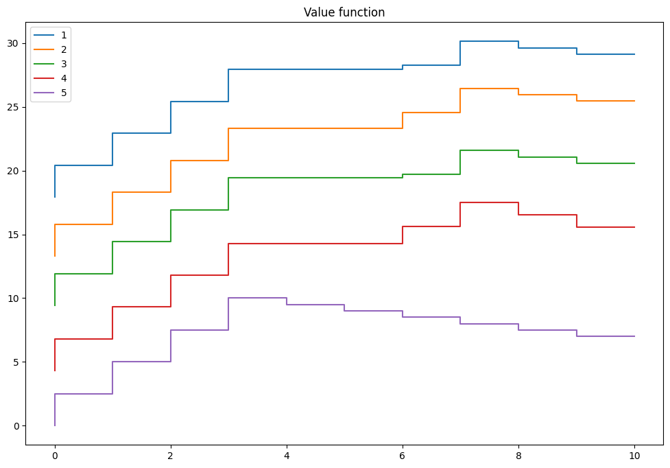
Time period 5

[[ 0.   0.   0.   0.   0. ]
 [ 0.   0.   0.   0.   2.5]
 [ 0.   0.   0.   0.   5. ]
 [ 0.   0.   0.   0.   7.5]
 [ 0.   0.   0.   0.  10. ]
 [ 0.   0.   0.   0.   9.5]
 [ 0.   0.   0.   0.   9. ]
 [ 0.   0.   0.   0.   8.5]
 [ 0.   0.   0.   0.   8. ]
 [ 0.   0.   0.   0.   7.5]
 [ 0.   0.   0.   0.   7. ]] 

Time period 4

[[ 0.     0.     0.     4.3    0.   ]
 [ 0.     0.     0.     6.8    2.5  ]
 [ 0.     0.     0.     9.3    5.   ]
 [ 0.     0.     0.    11.8    7.5  ]
 [ 0.     0.     0.    14.3   10.   ]
 [ 0.     0.     0.    14.3    9.5  ]
 [ 0.     0.     0.    14.3    9.   ]
 [ 0.     0.     0.    15.625  8.5  ]
 [ 0.     0.     0.    17.5    8.   ]
 [ 0.     0.     0.    16.525  7.5  ]
 [ 0.     0.     0.    15.55   7.   ]] 

Time period 3

[[ 0.     0.     9.425  4.3    0.   ]
 [ 0.     0.    11.925  6.8    2.5  ]
 [ 0.     0.    14.425  9.3    5.   ]
 [ 0.     0.    16.925 11.8    7.5  ]
 [ 0.     0.    19.425 14.3   10.   ]
 [ 0.     0.    19.425 14.3    9.5  ]
 [ 0.     0.    19.425 14.3    9.   ]
 [ 0.     0.    19.71  15.625  8.5  ]
 [ 0.     0.    21.585 17.5    8.   ]
 [ 0.     0.    21.085 16.525  7.5  ]
 [ 0.     0.    20.585 15.55   7.   ]] 

Time period 2

[[ 0.      13.30575  9.425    4.3      0.     ]
 [ 0.      15.80575 11.925    6.8      2.5    ]
 [ 0.      18.30575 14.425    9.3      5.     ]
 [ 0.      20.80575 16.925   11.8      7.5    ]
 [ 0.      23.30575 19.425   14.3     10.     ]
 [ 0.      23.30575 19.425   14.3      9.5    ]
 [ 0.      23.30575 19.425   14.3      9.     ]
 [ 0.      24.57875 19.71    15.625    8.5    ]
 [ 0.      26.45375 21.585   17.5      8.     ]
 [ 0.      25.95375 21.085   16.525    7.5    ]
 [ 0.      25.45375 20.585   15.55     7.     ]] 

Time period 1

[[17.9310625 13.30575    9.425      4.3        0.       ]
 [20.4310625 15.80575   11.925      6.8        2.5      ]
 [22.9310625 18.30575   14.425      9.3        5.       ]
 [25.4310625 20.80575   16.925     11.8        7.5      ]
 [27.9310625 23.30575   19.425     14.3       10.       ]
 [27.9310625 23.30575   19.425     14.3        9.5      ]
 [27.9310625 23.30575   19.425     14.3        9.       ]
 [28.2654625 24.57875   19.71      15.625      8.5      ]
 [30.1404625 26.45375   21.585     17.5        8.       ]
 [29.6404625 25.95375   21.085     16.525      7.5      ]
 [29.1404625 25.45375   20.585     15.55       7.       ]] 

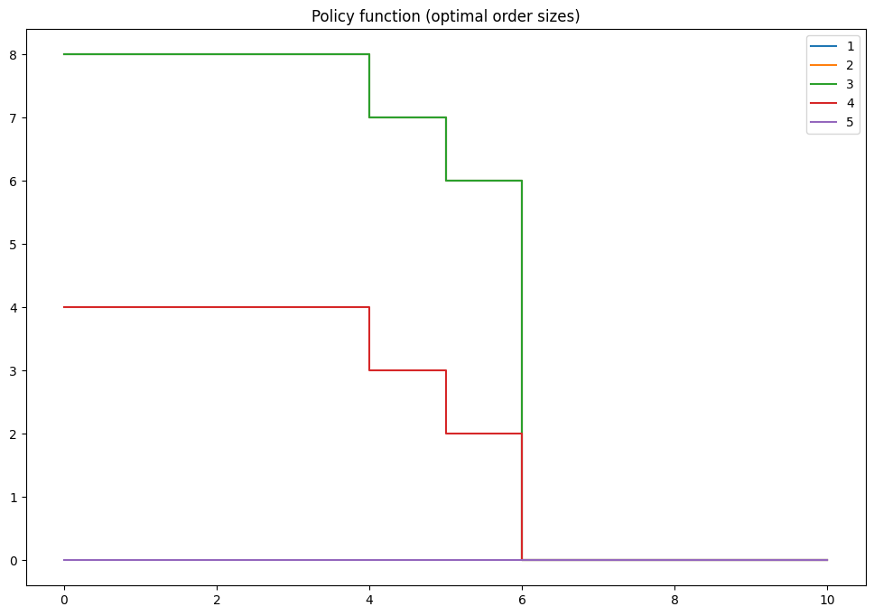
Optimal policy:
 [[8. 8. 8. 4. 0.]
 [8. 8. 8. 4. 0.]
 [8. 8. 8. 4. 0.]
 [8. 8. 8. 4. 0.]
 [8. 8. 8. 4. 0.]
 [7. 7. 7. 3. 0.]
 [6. 6. 6. 2. 0.]
 [0. 0. 0. 0. 0.]
 [0. 0. 0. 0. 0.]
 [0. 0. 0. 0. 0.]
 [0. 0. 0. 0. 0.]]

def plot_solution(model):
    plt.step(model.x,model.value)
    plt.legend([f'{i+1}' for i in range(model.value.shape[1])])
    plt.title('Value function')
    plt.show()
    plt.step(model.x,model.policy)
    plt.legend([f'{i+1}' for i in range(model.policy.shape[1])])
    plt.title('Policy function (optimal order sizes)')
    plt.show()
plot_solution(model)

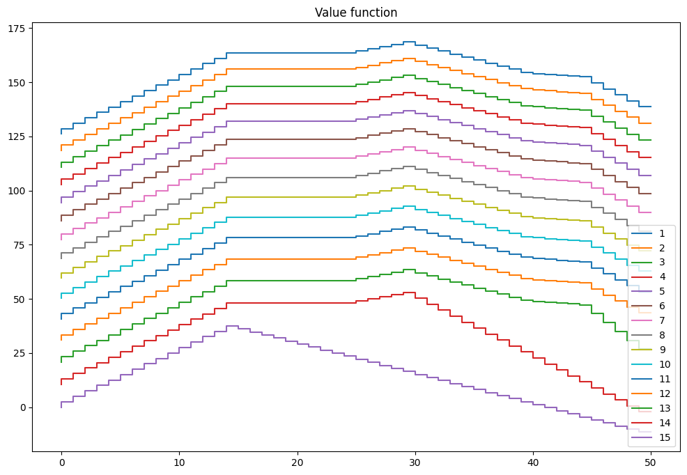
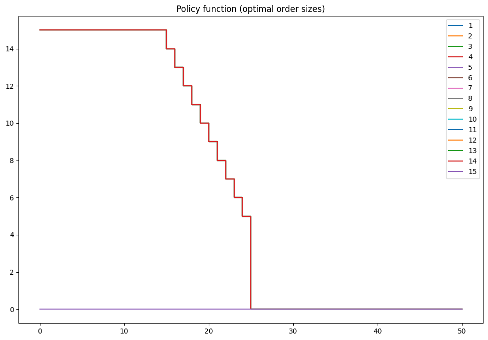
mod = inventory_model(label='production',max_inventory=50)
mod.demand = 15
mod.c = 5
mod.p = 2.5
mod.r = 1.4
mod.β = 0.975
mod = solver_backwards_induction(mod,T=15)
plot_solution(mod)

Contraction mappings and fixed points

Solution of a dynamic model in infinite horizon is the solution to the Bellman euqation which is an actual equation in function space

We rely on contraction properties of the Bellman operator to find the fixed point that in order to solve infinite horizon dynamic models

Definition

Let

• \( (S,\rho) \) be a complete metric space

• \( T: S \rightarrow S \) denote an operator mapping \( S \) to itself

\( T \) is called a contraction on \( S \) with modulus \( \lambda \) if \( 0 \le \lambda < 1 \) and

\[ \rho(Tx,Ty) \le \lambda \rho(x,y) \; \forall x,y \in S \]

Contraction mapping brings points in its domain “closer” to each other!

Example of contraction

\[\stackrel{\nearrow}{V} \quad \stackrel{\searrow}{c} \quad \stackrel{\searrow}{c} \quad \stackrel{\searrow}{c} \quad \dots\]

• interest rate \(r\)

• What is the value of the annuity \(V\)?

\[\stackrel{\nearrow}{V} \quad \stackrel{\searrow}{c} \quad \stackrel{\searrow}{c} \quad \stackrel{\searrow}{c} \quad \dots\]

\[V=\quad \frac{c}{(1+r)^0} + \quad \frac{c}{(1+r)^1} + \quad \frac{c}{(1+r)^2} + \quad \frac{c}{(1+r)^3} + \quad \dots\]

\[\beta = \frac{1}{1+r}\]

\[V=\quad c + \quad c \beta + \quad c \beta^2 + \quad c \beta^3 + \quad \dots = \sum_{t=0}^{\infty} \beta^t c\]

Assuming \(\beta<1\)

\[V = \sum_{t=0}^{\infty} \beta^t c = \frac{c}{1-\beta}\]

But we can also reformulate recursively (as “Bellman equation” without choice)

\[V = c + \beta ( c + \beta c + \beta^2 c + \dots ) = c + \beta V\]

\[T(V) = c + \beta V\]

\[|T(V_1) - T(V_2)| = |(c + \beta V_1) - (c + \beta V_2)| = \beta | V_1 - V_2 |\]

• contraction mapping under Euclidean norm!

• modulus \(\beta\)

Successive approximations to find the value of annuity

1. Start with a guess \(V_0\)

2. Insert into the “Bellman equation”

\[V_{i+1} = c + \beta V_i\]

3. Repeat until convergence

\[||V_{i}-V_{i-1}|| \le \varepsilon \text{ (small number)}\]

import numpy as np
import matplotlib.pyplot as plt
%matplotlib inline

class annuity():

    def __init__(self,c=1,beta=.9):
        self.c = c           # Annual payment
        self.beta = beta     # Discount factor
        self.analytic = c/(1-beta)  # compute analytic solution right away

    def bellman(self,V):
        '''Bellman equation'''
        return self.c + self.beta*V

    def solve(self, maxiter = 1000, tol=1e-4, verbose=False):
        '''Solves the model using successive approximations'''
        if verbose: print('{:<4} {:>15} {:>15}'.format('Iter','Value','Error'))
        V0=0
        for i in range(maxiter):
            V1=self.bellman(V0)
            if verbose: print('{:<4d} {:>15.8f} {:>15.8f}'.format(i,V1,V1-self.analytic))
            if abs(V1-V0) < tol:
                break
            V0=V1
        else:  # when i went up to maxiter
            print('No convergence: maximum number of iterations achieved!')
        return V1

a = annuity(c=10,beta=0.954)
print('Analytic solution is',a.analytic)
print('Numeric solution is ',a.solve())

Analytic solution is 217.3913043478259
Numeric solution is  217.38928066546833

a.solve(verbose=True)

Iter           Value           Error
0        10.00000000   -207.39130435
1        19.54000000   -197.85130435
2        28.64116000   -188.75014435
3        37.32366664   -180.06763771
4        45.60677797   -171.78452637
5        53.50886619   -163.88243816
6        61.04745834   -156.34384600
7        68.23927526   -149.15202909
8        75.10026860   -142.29103575
9        81.64565624   -135.74564811
10       87.88995605   -129.50134829
11       93.84701808   -123.54428627
12       99.53005524   -117.86124910
13      104.95167270   -112.43963164
14      110.12389576   -107.26740859
15      115.05819655   -102.33310779
16      119.76551951    -97.62578484
17      124.25630562    -93.13499873
18      128.54051556    -88.85078879
19      132.62765184    -84.76365251
20      136.52677986    -80.86452449
21      140.24654798    -77.14475636
22      143.79520678    -73.59609757
23      147.18062726    -70.21067708
24      150.41031841    -66.98098594
25      153.49144376    -63.89986058
26      156.43083735    -60.96046700
27      159.23501883    -58.15628552
28      161.91020797    -55.48109638
29      164.46233840    -52.92896595
30      166.89707083    -50.49423351
31      169.21980557    -48.17149877
32      171.43569452    -45.95560983
33      173.54965257    -43.84165178
34      175.56636855    -41.82493580
35      177.49031560    -39.90098875
36      179.32576108    -38.06554327
37      181.07677607    -36.31452828
38      182.74724437    -34.64405998
39      184.34087113    -33.05043322
40      185.86119106    -31.53011329
41      187.31157627    -30.07972808
42      188.69524376    -28.69606059
43      190.01526255    -27.37604180
44      191.27456047    -26.11674388
45      192.47593069    -24.91537366
46      193.62203788    -23.76926647
47      194.71542414    -22.67588021
48      195.75851463    -21.63278972
49      196.75362295    -20.63768140
50      197.70295630    -19.68834805
51      198.60862031    -18.78268404
52      199.47262377    -17.91868057
53      200.29688308    -17.09442127
54      201.08322646    -16.30807789
55      201.83339804    -15.55790631
56      202.54906173    -14.84224262
57      203.23180489    -14.15949946
58      203.88314187    -13.50816248
59      204.50451734    -12.88678701
60      205.09730954    -12.29399481
61      205.66283330    -11.72847104
62      206.20234297    -11.18896138
63      206.71703520    -10.67426915
64      207.20805158    -10.18325277
65      207.67648120     -9.71482314
66      208.12336307     -9.26794128
67      208.54968837     -8.84161598
68      208.95640270     -8.43490165
69      209.34440818     -8.04689617
70      209.71456540     -7.67673895
71      210.06769539     -7.32360895
72      210.40458141     -6.98672294
73      210.72597066     -6.66533369
74      211.03257601     -6.35872834
75      211.32507751     -6.06622683
76      211.60412395     -5.78718040
77      211.87033425     -5.52097010
78      212.12429887     -5.26700548
79      212.36658112     -5.02472322
80      212.59771839     -4.79358596
81      212.81822335     -4.57308100
82      213.02858507     -4.36271928
83      213.22927016     -4.16203419
84      213.42072373     -3.97058062
85      213.60337044     -3.78793391
86      213.77761540     -3.61368895
87      213.94384509     -3.44745926
88      214.10242822     -3.28887613
89      214.25371652     -3.13758783
90      214.39804556     -2.99325879
91      214.53573546     -2.85556888
92      214.66709163     -2.72421272
93      214.79240542     -2.59889893
94      214.91195477     -2.47934958
95      215.02600485     -2.36529950
96      215.13480863     -2.25649572
97      215.23860743     -2.15269692
98      215.33763149     -2.05367286
99      215.43210044     -1.95920391
100     215.52222382     -1.86908053
101     215.60820152     -1.78310283
102     215.69022425     -1.70108010
103     215.76847394     -1.62283041
104     215.84312414     -1.54818021
105     215.91434043     -1.47696392
106     215.98228077     -1.40902358
107     216.04709585     -1.34420850
108     216.10892944     -1.28237491
109     216.16791869     -1.22338566
110     216.22419443     -1.16710992
111     216.27788148     -1.11342286
112     216.32909894     -1.06220541
113     216.37796038     -1.01334396
114     216.42457421     -0.96673014
115     216.46904379     -0.92226055
116     216.51146778     -0.87983657
117     216.55194026     -0.83936409
118     216.59055101     -0.80075334
119     216.62738566     -0.76391869
120     216.66252592     -0.72877843
121     216.69604973     -0.69525462
122     216.72803144     -0.66327291
123     216.75854200     -0.63276235
124     216.78764906     -0.60365528
125     216.81541721     -0.57588714
126     216.84190802     -0.54939633
127     216.86718025     -0.52412410
128     216.89128996     -0.50001439
129     216.91429062     -0.47701373
130     216.93623325     -0.45507110
131     216.95716652     -0.43413783
132     216.97713686     -0.41416749
133     216.99618856     -0.39511578
134     217.01436389     -0.37694046
135     217.03170315     -0.35960120
136     217.04824481     -0.34305954
137     217.06402555     -0.32727880
138     217.07908037     -0.31222398
139     217.09344267     -0.29786167
140     217.10714431     -0.28416004
141     217.12021567     -0.27108868
142     217.13268575     -0.25861860
143     217.14458221     -0.24672214
144     217.15593142     -0.23537292
145     217.16675858     -0.22454577
146     217.17708768     -0.21421666
147     217.18694165     -0.20436270
148     217.19634234     -0.19496201
149     217.20531059     -0.18599376
150     217.21386630     -0.17743805
151     217.22202845     -0.16927590
152     217.22981514     -0.16148921
153     217.23724365     -0.15406070
154     217.24433044     -0.14697391
155     217.25109124     -0.14021311
156     217.25754104     -0.13376331
157     217.26369415     -0.12761019
158     217.26956422     -0.12174013
159     217.27516427     -0.11614008
160     217.28050671     -0.11079764
161     217.28560340     -0.10570095
162     217.29046565     -0.10083870
163     217.29510423     -0.09620012
164     217.29952943     -0.09177492
165     217.30375108     -0.08755327
166     217.30777853     -0.08352582
167     217.31162072     -0.07968363
168     217.31528616     -0.07601818
169     217.31878300     -0.07252135
170     217.32211898     -0.06918537
171     217.32530151     -0.06600284
172     217.32833764     -0.06296671
173     217.33123411     -0.06007024
174     217.33399734     -0.05730701
175     217.33663346     -0.05467089
176     217.33914832     -0.05215603
177     217.34154750     -0.04975685
178     217.34383631     -0.04746803
179     217.34601984     -0.04528450
180     217.34810293     -0.04320142
181     217.35009020     -0.04121415
182     217.35198605     -0.03931830
183     217.35379469     -0.03750966
184     217.35552013     -0.03578421
185     217.35716621     -0.03413814
186     217.35873656     -0.03256779
187     217.36023468     -0.03106967
188     217.36166388     -0.02964046
189     217.36302735     -0.02827700
190     217.36432809     -0.02697626
191     217.36556900     -0.02573535
192     217.36675282     -0.02455153
193     217.36788219     -0.02342216
194     217.36895961     -0.02234474
195     217.36998747     -0.02131688
196     217.37096805     -0.02033630
197     217.37190352     -0.01940083
198     217.37279595     -0.01850839
199     217.37364734     -0.01765701
200     217.37445956     -0.01684479
201     217.37523442     -0.01606993
202     217.37597364     -0.01533071
203     217.37667885     -0.01462550
204     217.37735162     -0.01395272
205     217.37799345     -0.01331090
206     217.37860575     -0.01269860
207     217.37918989     -0.01211446
208     217.37974715     -0.01155720
209     217.38027878     -0.01102557
210     217.38078596     -0.01051839
211     217.38126980     -0.01003454
212     217.38173139     -0.00957295
213     217.38217175     -0.00913260
214     217.38259185     -0.00871250
215     217.38299262     -0.00831172
216     217.38337496     -0.00792938
217     217.38373971     -0.00756463
218     217.38408769     -0.00721666
219     217.38441965     -0.00688469
220     217.38473635     -0.00656800
221     217.38503848     -0.00626587
222     217.38532671     -0.00597764
223     217.38560168     -0.00570267
224     217.38586400     -0.00544035
225     217.38611426     -0.00519009
226     217.38635300     -0.00495135
227     217.38658076     -0.00472358
228     217.38679805     -0.00450630
229     217.38700534     -0.00429901
230     217.38720309     -0.00410125
231     217.38739175     -0.00391260
232     217.38757173     -0.00373262
233     217.38774343     -0.00356092
234     217.38790723     -0.00339711
235     217.38806350     -0.00324085
236     217.38821258     -0.00309177
237     217.38835480     -0.00294955
238     217.38849048     -0.00281387
239     217.38861992     -0.00268443
240     217.38874340     -0.00256095
241     217.38886121     -0.00244314
242     217.38897359     -0.00233076
243     217.38908080     -0.00222354
244     217.38918309     -0.00212126
245     217.38928067     -0.00202368

217.38928066546833

Solving infinite horizon dynamic models

1. Value function iterations = successive approximations on the Bellman operator \(\rightarrow\) to solve for the fixed point of Bellman operator

2. Policy iteration method = Howard’s policy improvement algorithm, iterative solution for the fixed point of Bellman operator

3. Newton-Kantorovich method = Newton solver for the fixed point of Bellman operator, mathematically identical to Howard’s iterations

Convergence of infinite horizon solution methods

• In infinite horizon all solution methods continue until convergence.

• How can we be sure that the algorithm would terminate?

The answer is given by the theory of contraction mappings:

• Bellman operator is generally a contraction mapping

• Banach theorem guarantees uniqueness of the fixed point, and

• Successive approximation solver is globally convergent (works with any starting point)

Banach contraction mapping theorem (fixed point theorem)

Let \((S,\rho)\) be a complete metric space with a contraction mapping \(T: S \rightarrow S\). Then

1. \(T\) admits a unique fixed-point \(V^{\star} \in S\), i.e. \(T(V^{\star}) = V^{\star}\).

2. \(V^{\star}\) can be found by repeated application of the operator \(T\), i.e. \(T^n(V) \rightarrow V^{\star}\) as \(n\rightarrow \infty\).

In other words, the fixed point can be found by successive approximations from any starting point \(\rightarrow\) VFI method follows

What about Bellman operator?

\[T(V)(\text{state}) = \max_{\text{decisions}} \big[ U(\text{state},\text{decision}) + \beta \mathbb{E}\big\{ V(\text{next state}) \big| \text{state},\text{decision} \big\} \big]\]

• Bellman operator \(T: U \rightarrow U\) from functional space \(U\) to itself

• metric space \((U,d_{\infty})\) with uniform/infinity/sup norm (max abs distance between functions over their domain)

Blackwell sufficient conditions for contraction

Let \(X \subseteq \mathbb{R}^n\) and \(B(x)\) be the space of bounded functions \(f: X \rightarrow \mathbb{R}\) defined on \(X\). Suppose that \(T: B(X) \rightarrow B(X)\) is an operator satisfying the following conditions:

1. (monotonicity) For any \(f,g \in B(X)\) and \(f(x) \le g(x)\) for all \(x\in X\) implies \(T(f)(x) \le T(g)(x)\) for all \(x\in X\),

2. (discounting) There exists \(\beta \in (0,1)\) such that

\[T(f+a)(x) \le T(f)(x) + \beta a, \text{ for all } f\in B(X), a \ge 0, x\in X,\]

Then \(T\) is a contraction mapping with modulus \(\beta\).

• Monotonicity of Bellman equation follows trivially due to maximization in \(T(V)(x)\)

• Discounting: satisfied by elementary argument when \(\beta<1\)

Under additional boundedness conditions, Bellman operator is a contraction mapping by Blackwell sufficient conditions

\(\Rightarrow\)

• unique solution

• VFI algorithm is globally convergent

• does not depend on the numerical implementation of the Bellman operator

Why do we need other solution algorithms?

Although VFI is guaranteed to find the solution, it may be very inefficient when modulus of contraction (discount factor \(\beta\)) is close to one.

• Newton-based method converge quadratically, but are not globally convergent, have to be initialized at their domain of attraction

• Polyalgorithm would be a good idea, see NFXP in the next lecture

Inventory dynamics problem with stochastic demand in infinite time

The model is given by the Bellman equation

\[\begin{split} \begin{array}{rcl} V(x_t,d_t) &=& \max_{q_t \ge 0} \Big\{ \pi_t + \beta \mathbb{E}\Big[ V\big(x_{t+1} , d_{t+1} \big) \Big| x_t,d_t,q_t \Big] \Big\} \\ &=& \max_{q_t \ge 0} \Big\{ s_t p - k_t r - c \mathbb{1}\{q_t>0\} + \beta \mathbb{E}\Big[ V\big( k_t, d_{t+1} \big) \Big] \Big\} \end{array} \end{split}\]

\[\begin{split} \begin{array}{rcl} s_t &=& \min\{x_t,d_t\} \\ k_t &=& \max\{x_t-d_t,0\} + q_t \end{array} \end{split}\]

Dropping the time subscripts

Because we’ll be solving the problem in infinite horizon, the time subscripts can be dropped, and we can just have current period variables \( x,d,q,s,k \), and next period variables denoted by prime, i.e. \( x' \)

The Bellman equation is then

\[\begin{split} \begin{array}{rcl} V(x,d) &=& \max_{q \ge 0} \Big\{ \pi + \beta \mathbb{E}\Big[ V\big(x', d' \big) \Big| x,d,q \Big] \Big\} \\ &=& \max_{q \ge 0} \Big\{ s\cdot p - k\cdot r - c \mathbb{1}\{q>0\} + \beta \mathbb{E}\Big[ V\big( k, d' \big) \Big] \Big\} \end{array} \end{split}\]

\[\begin{split} \begin{array}{rcl} s &=& \min\{x,d\} \\ k &=& \max\{x-d,0\} + q \end{array} \end{split}\]

Bellman equation in expected value function space

Note that similar to the bus engine replacement model, the inventory model features random variable which distribution does not depend on the previous period variables (it is idiosyncratic).

In this case it is possible to reduce the dimensionality of the fixed point problem by rewriting the Bellman operator in expected value function terms.

\[ EV(x') = \mathbb{E}\Big[ V\big(x', d' \big) \Big| x,d,q \Big] = \mathbb{E}\Big[ V\big(x', d' \big) \Big], \]

where the expectation is taken over the distribution of the next period demand \( d' \). The conditioning on \( x,d,q \) can be dropped exactly because \( d' \) is idiosyncratic.

We can then write the Bellman equation as

\[ V(x,d) = \max_{q \ge 0} \Big\{ s\cdot p - k\cdot r - c \mathbb{1}\{q>0\} + \beta EV(k) \Big\} \]

\[ V(x,d) = \max_{q \ge 0} \Big\{ p \min\{x,d\} - r ( \max\{x-d,0\} + q ) - c \mathbb{1}\{q>0\} + \beta EV(\max\{x-d,0\} + q) \Big\} \]

Taking the expectation with respect to \( d \) on both sides, we get

\[ EV(x) = \mathbb{E}\Big[ \max_{q \ge 0} \Big\{ p \min\{x,d\} - r ( \max\{x-d,0\} + q ) - c \mathbb{1}\{q>0\} + \beta EV(\max\{x-d,0\} + q) \Big\} \Big] \]

By assumption the inventory is discrete, and so it is natural to assume that the demand is also represented as a discrete random variable. Then the expectation can be written as a sum weighted with the corresponding probabilities \( pr(d) \), as

\[ EV(x) = \sum_{d} \Big[ \max_{q \ge 0} \Big\{ p \min\{x,d\} - r ( \max\{x-d,0\} + q ) - c \mathbb{1}\{q>0\} + \beta EV(\max\{x-d,0\} + q) \Big\} \Big] pr(d) \]

This is functional equation in \( EV \) which is also a contraction mapping!

Origin of the term Dynamic Programming

The 1950’s were not good years for mathematical research. We had a very interesting gentleman in Washington named Wilson. He was Secretary of Defence, and he actually had a pathological fear and hatred of the word “research”. I’m not using the term lightly; I’m using it precisely. His face would suffuse, he would turn red, and he would get violent if people used the term, research, in his presence. You can imagine how he felt, then, about the term, mathematical. Hence, I felt I had to do something to shield Wilson and the Air Force from the fact that I was really doing mathematics inside the RAND Corporation.

What title, what name, could I choose?

In the first place, I was interested in planning, in decision-making, in thinking. But planning, is not a good word for various reasons. I decided therefore to use the word, “programming”. I wanted to get across the idea that this was dynamic, this was multistage, this was time-varying.

I thought, let’s kill two birds with one stone. Let’s take a word which has an absolutely precise meaning, namely dynamic, in the classical physical sense. It also has a very interesting property as an adjective, and that is it’s impossible to use the word, dynamic, in the pejorative sense.

Thus, I thought dynamic programming was a good name. It was something not even a Congressman could object to. So I used it as an umbrella for my activities.

— 📖 Bellman’s autobiography “The Eye of the Hurricane”

References and Additional Resources

• 📖 Rust [2016] “Dynamic programming”, The New Palgrave Dictionary of Economics

• 📖 Adda and Cooper [2023], “Dynamic Economics: Quantitative Methods and Applications”, chapters 2 and 3

• 📖 Aguirregabiria and Mira [2010] “Dynamic discrete choice structural models: A survey”

• Wiki: Bellman equation https://en.wikipedia.org/wiki/Bellman_equation

• Computer science view on DP link

• “Knowing When to Stop” by Theodore Hill, American Scientist link