📖 CCP-Based Estimation

⏱ | words

References

Integrated \(\ne\) expected value function

Maintain the setup of from the Zurcher engine replacement model of Rust [1987], leaning to more generality..

The Bellman equation of the Zurcher problem is

\[V(x,\varepsilon) = \max_{d\in D(x)} \Big\{ \underbrace{u(x,d) + \beta \int_{X} \Big( \int_{\Omega} V(x',\varepsilon') q(\varepsilon'|x') d\varepsilon'\Big) \pi(x'|x,d) dx'}_{v(x,d)} + \varepsilon_d \Big\}\]

\[ V(x,\varepsilon) = \max_{d\in D(x)} \big\{ v(x,d) + \varepsilon_{d} \big\} \]

\[ v(x,d) = u(x,d) + \beta EV(x,d) \]

\[ EV(x,d) = \int_{X} \log \big( \exp[v(x',0)] + \exp[v(x',1)] \big) \pi(x'|x,d) dx' \]

The last equation uses the EV1 assumption on the distribution of \(\varepsilon\), but in more generality can be written as

\[ EV(x,d) = \int_{X} \int_{\Omega} V(x',\varepsilon') q(\varepsilon'|x') \pi(x'|x,d) d\varepsilon' dx' \]

Let’s repeat the terminology:

• \(v(x,d)\) is choice-specific value function or conditional value function

• \(EV(x,d)\) is commonly referred to as the expected value function and sometimes as ex-post value function

And here is a new object and yet another representation

• \(V_\sigma(x)\) is the integrated value function also known as the ex-ante value function

  • \(\sigma\) is involved following the notation of Aguirregabiria and Mira [2007] who define it as the value function under a strategy profile \(\sigma\)

\[ V_\sigma(x) = \int_{\Omega} V(x,\varepsilon) q(\varepsilon|x) d\varepsilon \]

\[ EV(x,d) = \int_{X} V_\sigma(x') \pi(x'|x,d) dx' \]

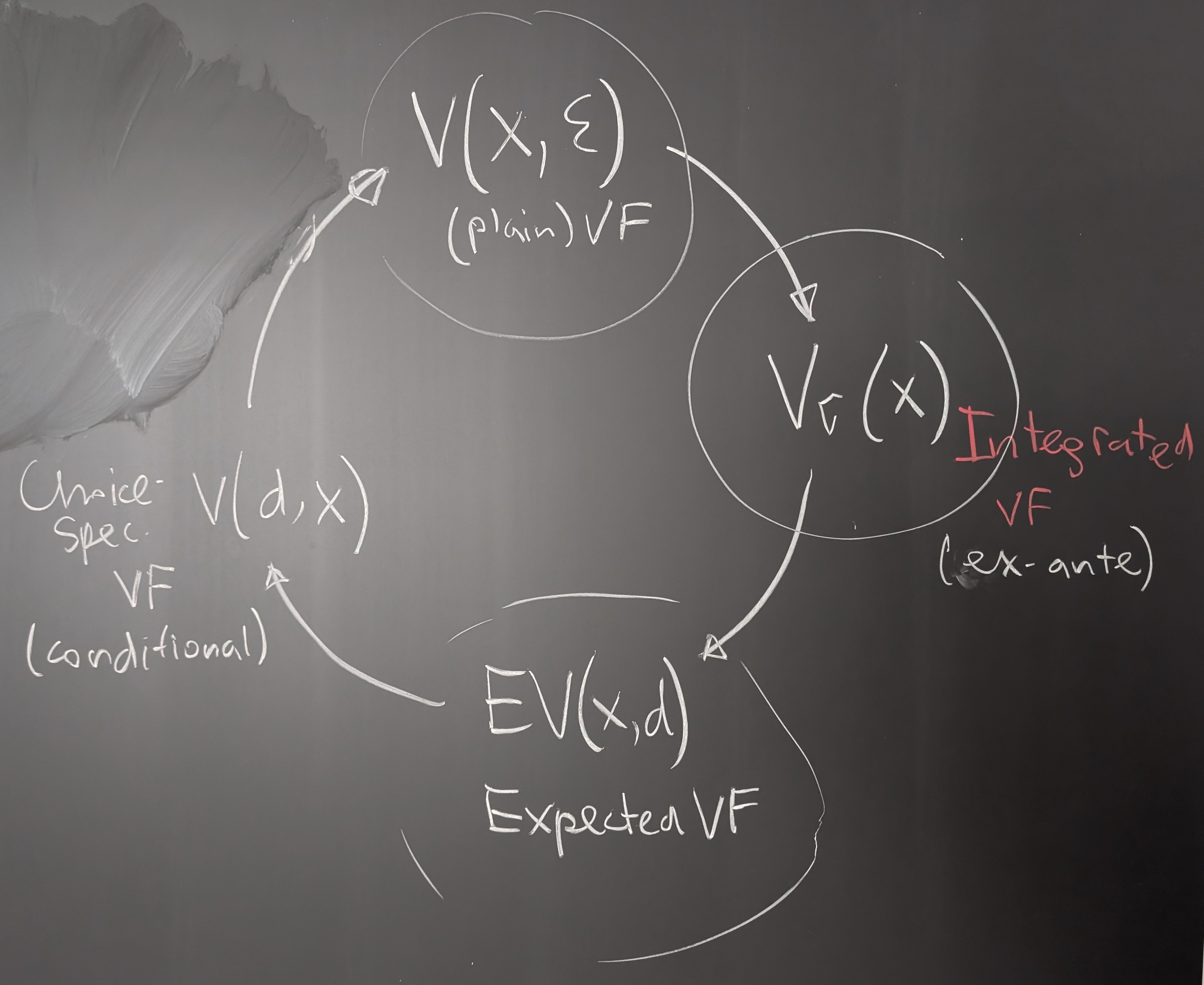
Fig. 1 The Bellman circle of value functions: plain value function \(V(x,\varepsilon)\), integrated value function \(V_\sigma(x)\), expected value function \(EV(x,d)\) and choice-specific value function \(v(x,d)\)

We could write the Bellman equation in the space of integrated value functions \(V_\sigma(x)\) by cutting the circle of Bellman at a different point:

\(\dots\) \(\rightarrow\) \(V(x,\varepsilon)\) \(\rightarrow\) \(V_\sigma(x)\) \(\rightarrow\) \(EV(x)\) \(\rightarrow\) \(v(x,d)\) \(\rightarrow\) \(V(x,\varepsilon)\) \(\rightarrow\) \(\dots\)

The new representation of the Bellman equation is:

\[ V_\sigma(x) = \int_{\Omega} \max_{d'\in D(x)} \Big\{ \underbrace{u(x,d') + \beta \int_{X} V_\sigma(x') \pi(x'|x,d') dx'}_{v(x,d')} + \varepsilon_{d'} \Big\} q(\varepsilon|x) d\varepsilon \]

\[ V_\sigma(x) = \int_{\Omega} \max_{d'\in D(x)} \left\{ v(x,d') + \varepsilon_{d'} \right\} q(\varepsilon|x) d\varepsilon \]

This is the expectation of the maximum utility in RUM with alternative utilities given by \(v(x,d') + \varepsilon_{d'}\)!

McFadden [1974] called this function the Social Surplus Function.

In the EV1 case we simply have due to max-stability, with \(\gamma \approx 0.5772\) being the Euler-Mascheroni constant

\[ V_\sigma(x) = \log \big( \sum_{d' \in D(x)} \exp[v(x,d')] \big) + \gamma \]

Choice probabilities

Recall that by the Williams-Daly-Zachary Theorem in the general case the choice probabilities can be written as

\[ P(d|x) = \frac{\partial}{\partial v(x,d)} \mathbb{E}\left\{\max_{d' \in D(x)} \big[ v(d',x) +\varepsilon(d') \big]\Big|x\right\} = \frac{\partial V_\sigma(x)}{\partial v(x,d)} \]

And under EV1 assumption

\[ P(d|x) = \frac{\partial \log \big( \sum_{d' \in D(x)} \exp[v(x,d')] \big)}{\partial v(x,d)} = \frac{\exp[v(x,d)]}{\sum_{d'\in D(x)} \exp[v(x,d')]} \]

Inversion theorem

📖 Hotz and Miller [1993] “Conditional Choice Probabilities and the Estimation of Dynamic Models”

Let \(d_0\) denote the reference alternative \(\rightarrow\) the values of other alternatives will be measured relative to it

Why?

For each \(x\) consider the vector of value differences \(\Delta v(d,x) \in \mathbb{R}^{K-1}\) where \(K=|D(x)|\) is the number of alternatives. The elements of this vector are

\[ \Delta v(x,d) = v(x,d) - v(x,d_0), \quad d \in D(x)\setminus\{d_0\} \]

Another way to express the choice probabilities \(P(d|x)\) is through the integral with respect to the distribution of \(q(\varepsilon|x)\)

\[ P(d|x)= \int_\Omega I\left\{ d = \arg\max_{d' \in D(x)} \{v(x,d')+\varepsilon_{d'}\} \right\}q(\varepsilon|x) d\varepsilon = \]

\[ = \int_\Omega I\left\{ \varepsilon_{d'} \leqslant v(x,d) - v(x,d') + \varepsilon_{d}, \forall d' \in D(x)\setminus\{d\} \right\}q(\varepsilon|x) d\varepsilon = \]

\[ = \int_\Omega I\left\{ \varepsilon_{d'} \leqslant \Delta v(x,d) - \Delta v(x,d') + \varepsilon_{d}, \forall d' \in D(x)\setminus\{d\} \right\}q(\varepsilon|x) d\varepsilon = \]

\[ = \int_{\{\varepsilon:\; \varepsilon_{d'} \leqslant \Delta v(x,d) - \Delta v(x,d') + \varepsilon_{d}, \forall d' \in D(x)\setminus\{d\}\}} q(\varepsilon|x) d\varepsilon = Q_{d}(\Delta v(x),x) \]

Compare this derivation to: Static multinomial logit model

In other words if

\[ Q_d: \mathbb{R}^{K-1} \ni \delta \mapsto P \in [0,1]^{K} \]

is a mapping from \(K-1\) value differences to the \(K\) vector of probabilities, then the choice probabilities are given by

\[ P(x) = Q_{d}(\Delta v(x),x) \]

Inversion Theorem

Under certain regularity conditions on \(q(\varepsilon|x)\) the mapping \(Q_d\) is invertible, i.e. there exists a mapping \(Q_d^{-1}: [0,1]^{K} \ni P \mapsto \delta \in \mathbb{R}^{K-1}\) such that

\[ \Delta v(x) = Q_d^{-1}(P(x),x) \]

Example

In the multinomial logit case for some \(d_0 \in D(x)\)

\[ P(d|x) = \frac{\exp[v(x,d)]}{\sum_{d'\in D(x)} \exp[v(x,d')]} = \frac{\exp[\Delta v(x,d)]}{1+\sum_{d'\in D(x)\setminus\{d_0\}} \exp[\Delta v(x,d')]}, \]

\[ P(d_0|x) = \frac{1}{1+\sum_{d'\in D(x)\setminus\{d_0\}} \exp[\Delta v(x,d')]} \]

The inverse map is given by

\[ \frac{P(d|x)}{P(d_0|x)} = \exp[\Delta v(x,d)] \implies \]

\[ \Delta v(x,d) = \log P(d|x) - \log P(d_0|x), \quad d \in D(x)\setminus\{d_0\} \]

What we have:

• Hotz-Miller inversion gives a mapping from the choice probabilities to the value differences for any choice model with random terms \(\varepsilon\) satisfying the regularity conditions of the theorem

• In the EV1 and GEV cases we have a closed-form expressions for the inverse map

Relationship between \(V_\sigma(x)\), \(v(x,d)\) and choice probabilities

Recall that the choice probability \(P(d|x)\) in general case are simply the expectation of the indicator that a particular choice \(d\) maximizes yields maximum utility

\[ P(d|x)= \hbox{Prob}\left\{d = \arg\max_{d' \in D(x)} \{v(x,d')+\varepsilon_{d'}\}|x\right\} = \]

\[ = \int_\Omega I\left\{ d = \arg\max_{d' \in D(x)} \{v(x,d')+\varepsilon_{d'}\} \right\}q(\varepsilon|x) d\varepsilon = \]

\[ = \mathbb{E}\left[\left. I\left\{ d = \arg\max_{d' \in D(x)} \{v(x,d')+\varepsilon_{d'}\} \right\} \right|x \right] \]

The last expression for \(V_\sigma(x)\) can be expanded using the law of iterated expectations as

\[ V_\sigma(x) = \int_{\Omega} \max_{d'\in D(x)} \left\{ v(x,d') + \varepsilon_{d'} \right\} q(\varepsilon|x) d\varepsilon = \mathbb{E}\left[ \max_{d'\in D(x)} \left\{ v(x,d') + \varepsilon_{d'} \right\} \right] = \]

\[ = \sum_{d \in D(x)} P(d|x) \mathbb{E}\left[\left. \max_{d'\in D(x)} \left\{ v(x,d') + \varepsilon_{d'} \right\} \right| d = \arg\max_{d''\in D(x)} \{v(x,d'')+\varepsilon_{d''}\} \right] = \]

\[ = \sum_{d \in D(x)} P(d|x) \mathbb{E}\left\{ v(x,d) + \varepsilon_{d} \left| d = \arg\max_{d''\in D(x)} \{v(x,d'')+\varepsilon_{d''}\} \right.\right\} = \]

\[ = \sum_{d \in D(x)} P(d|x)\left[ v(x,d) + \mathbb{E}\left\{ \varepsilon_{d} \left| d = \arg\max_{d''\in D(x)} \{v(x,d'')+\varepsilon_{d''}\} \right.\right\}\right] \]

The term

\[ e(x,d) = \mathbb{E}\left\{ \varepsilon_{d} \left| d = \arg\max_{d''\in D(x)} \{v(x,d'')+\varepsilon_{d''}\} \right.\right\} \]

has special name of correction term, see Arcidiacono and Miller [2011], which is equal the expectation of the random component conditional on the event that the alternative it is associated with has the highest value. We end up with

\[ V_\sigma(x) = \sum_{d \in D(x)} P(d|x) \big( v(x,d) + e(x,d) \big) \]

We can make one more step, using the Hotz-Miller inversion with a reference alternative \(d_0\), to arrive at

\[ V_\sigma(x) - v(d_0,x) = \sum_{d \in D(x)} P(d|x) \big( \Delta v(x,d) + e(x,d) \big) = \]

\[ = \sum_{d \in D(x)\setminus \{d_0\}} P(d|x) Q_d^{-1}(P(x),x,d) + \sum_{d \in D(x)} P(d|x) e(x,d) = \psi(d,x) \]

where \(\psi(d,x)\) is a function of the choice probabilities and not the value functions as shown by Arcidiacono and Miller [2011]

In other words, the difference between the integrated value function and any choice-specific reference value is a function of the choice probabilities only!

Special case of EV1 and GEV

Arcidiacono and Miller [2011] show that

\[ \text{EV1} \;\implies\;e(x,d) = \gamma-\log P(d|x) \]

\[ \text{GEV} \;\implies\;e(x,d) = \gamma - \sigma\log P(d| x) -(1-\sigma)\log\sum_{d' \in N(d)} P(d'|x) \]

where \(N(d)\) is the set of alternatives in the same nest as \(d\) and \(\gamma\leqslant 1\) is the EV scale parameters within the nest.

Some words on identification

Previous results have immediate implications for identification of the model primitives for the dynamic discrete choice models in general

We are interested in non-parametric identification of the model primitives \(\{u, \pi, q, \beta)\) given the data on \((x,d)\)

Here is a brief sketch

Assume discrete state space \(\rightarrow\) integral over \(\pi(x'|x,d)\) is a sum and can be represented by a matrix multiplication. Denote \(\Pi(d)\) the transition probability matrix for the state space \(X\) under action \(d\).

First, we can consistently estimate the choice probabilities \(P(d|x)\) — CCPs — and the transition probabilities \(\Pi(d)\) from the data on \((x,d)\) in the fist stage, giving the name to the corresponding CCP-based estimation methods.

Then, fix the reference alternative \(d_0\) and set \(u(d_0,x) = 0\) for all \(x\).

Stack all entities into vectors over the state space \(X\) to obtain

\[ v(d_0) = \underbrace{u(d_0)}_{=0} + \beta \Pi(d_0) V_\sigma \]

From the relationship between \(V_\sigma(x)\) and \(v(x,d)\) we have

\[ V_\sigma - \psi(d_0) = \beta \Pi(d_0) V_\sigma \implies V_\sigma = [I - \beta \Pi(d_0)]^{-1} \psi(d_0) \]

• This is an expression for the integrated function that only depends on objects we can estimate in a first stage

To non-parametrically estimate the utility function for the other actions, follow

\[ v(d) = u(d) + \beta \Pi(d) V_\sigma \]

\[ V_\sigma - \psi(p) = u(d) + \beta \Pi(d) V_\sigma \]

\[ u(d) = -\psi(p) + [I - \beta \Pi(d)] V_\sigma \]

\[ u(d) = -\psi(p) + [I - \beta \Pi(d)][I - \beta \Pi(d_0)]^{-1} \psi_0(p) \]

• Given \(\beta\) and \(q\) the utility function \(u(d)\) seem to be non-parametrically identified for all \(d \in D(x)\)

However, if we don’t assume \(u(d_0)=0\) and run through the same derivation again, we will end up with

\[ u(d) = -\psi(p) + [I - \beta \Pi(d)][I - \beta \Pi(d_0)]^{-1} \big(\psi_0(p)+u(d_0)\big) \]

and the obtained values of \(u(d)\) will perfectly consistent with the observed data informing \(P(d|x)\) and \(\Pi(d)\)!

• Normalization is needed unless some data informs the level of utility (e.g. data on costs or prices)

• We may also resort to parameterized utility function

Side note: Normalizing the value of an alternative to zero is common but not innocuous, see Kalouptsidi et al. [2021]

Finite dependence

Finite dependence is a powerful idea that helps identification and estimation

• In many applications there may be different paths from a points in the state space \(x_1\) and time period \(t_1\) to he point \(x_2\) and time period \(t_2\)

• Two different paths require different sequences of choices

• Yet, at \(x_2\) and time period \(t_2\) the future should look exactly the same regardless of the path taken to get there

\(\implies\)

The expected values at \(t_2\) can be differenced out \(\rightarrow\) resulting in a finite structure of dependence with no need for matrix inversions!

Similar to finite horizon problems.

Example

Zurcher model has one-period finite dependence!

Indeed, all regenerative models have this property: renewing today leads to exactly same future outlook as renewing one period later (and here exact time subscripts do not matter due to stationarity)

CCP-based estimation

There are many estimation approaches based on the CCP representation of the dynamic discrete choice models

• Minimum distance [Altuğ and Miller, 1998]

• Simulated moments [Hotz et al., 1994]

• Asymptotic least squares [Pesendorfer and Schmidt-Dengler, 2008]

• Quasi-maximum likelihood [Hotz and Miller, 1993]

• Pseudo-maximum likelihood [Aguirregabiria and Mira, 2002]

• Nested pseudo-likelihood [Aguirregabiria and Mira, 2007]

• Many-many more

Common scheme:

1. Estimate the CCPs \(P(d|x)\) and transition probabilities \(\Pi(d)\) directly from the data on \((x,d)\)

• Non-parametrically like frequency counts

• Parametrically like multinomial logit or nested logit for \(P(d|x)\) and discrete choice model for \(\Pi(d)\)

• Semi-parametrically like flexible or local logit

2. Use the estimated CCPs and transition probabilities to construct a criterion function that depends on the structural parameters of the model \(\theta\)

3. Optimize the criterion function to obtain the estimates \(\hat{\theta}\) by one of the above approaches

What are the strengths of CCP-based estimation? How does it compare to NFXP?

What are potential weaknesses and difficulties of this approach?

Quasi-likelihood estimation

Like all CCP-based methods, the quasi-likelihood estimation starts with the consistent estimation of the CCPs and transition probabilities from the data. Let’s focus on the specification of the statistical criterion for the second stage. Return to

\[ V_\sigma(x) = \sum_{d \in D(x)} P(d|x) \big( v(x,d) + e(x,d) \big) \]

Using the definition of the choice-specific value functions we have

\[ V_\sigma(x) = \sum_{d \in D(x)} P(d|x) \left( u(x,d) + \beta \int_{X} V_\sigma(x') \pi(x'|x,d) dx' + e(x,d) \right)= \]

\[ = \sum_{d \in D(x)} P(d|x) \left[ u(x,d) + e(x,d) \right] + \beta \sum_{d \in D(x)} P(d|x) \int_{X} V_\sigma(x') \pi(x'|x,d) dx' \]

Again, assuming discrete state space and stacking \(V_\sigma(x)\), \(P(d|x)\), \(u(x,d)\) and \(e(x,d)\) across the state space to form column vectors, we can write the last equation for every point of the state space in a matrix form

\[ V_\sigma = \sum_{d \in D(x)} P(d) \ast \left[ u(d) + e(d) \right] + \beta \sum_{d \in D(x)} P(d) \ast \Pi(d) V_\sigma \]

where \(\ast\) is the element-wise (Hadamard) product of vectors. Let

\[ \Pi = \sum_{d \in D(x)} P(d) \ast \Pi(d) \]

be a \(|X|\times|X|\) unconditional transition matrix, and denote \(I\) again the identity matrix of the same size, then

\[ V_\sigma = [I - \beta \Pi]^{-1} \sum_{d \in D(x)} P(d) \ast \left[ u(d) + e(d) \right] \]

Recall that the correction term \(e(d)\) is a function of the CCPs only, and therefore we can introduce an operator

\[ \varphi : [0,1]^{|X|\times|D|} \ni P \mapsto V_\sigma \in \mathbb{R}^{|X|} \]

that maps the CCPs into the integrated value functions.

Finally, denote

\[ \Lambda: \mathbb{R}^{|X|} \ni V_\sigma \mapsto \{P(d|x)\} \in \mathbb{R}^{|X|\times|D|} \]

the mapping from the integrated value functions to the CCPs given by the choice probability formulas above, which in the simple EV1 case take the form of multinomial logit

\[ \Lambda(V_\sigma) = \left\{\frac{\exp[u(x,d) + \beta \Pi(d) V_\sigma]}{\sum_{d'\in D(x)} \exp[u(x,d') + \beta \Pi(d') V_\sigma)]} \right\}_{d \in D(x), x \in X} \]

Following Aguirregabiria and Mira [2007] we define the composition operator as

\[ \Psi = \Lambda \circ \varphi : [0,1]^{|X|\times|D|} \ni P \mapsto \Lambda(\varphi(P)) \in [0,1]^{|X|\times|D|} \]

which maps the CCPs into the CCPs through the integrated value functions.

Note that \(\Psi\) depends on the structural parameters of the model \(\theta\) through \(u(x,d)\) and \(\beta\)

Resulting algorithm:

1. First stage CCPs and transition probabilities estimates \(\hat{P}(d|x)\) and \(\hat{\Pi}(d)\) for all \(x\) and \(d\)

2. Specify a quasi-likelihood function based on the estimated CCPs and transition probabilities

\[ \hat{P} \mapsto \Psi(\hat{P},\theta) \rightarrow \text{quasi-likelihood function} \]

where \(\Psi(\hat{P},\theta)\) is an operator given above. The quasi-likelihood function can be specified as

\[ \ell_n(\theta) = \log \mathcal{L}_n(\theta) = \sum_{i=1}\sum_{t} \log \Psi(\hat{P},\theta)(d_{i,t}|x_{i,t})\]

and the quasi-maximum likelihood estimator is given by

\[\hat{\theta}_{QML} = \arg\max_{\theta} \ell_n(\theta)\]

Swapping NFXP: NPL estimator

📖 Aguirregabiria and Mira [2002] “Swapping the Nested Fixed Point Algorithm: A Class of Estimators for Discrete Markov Decision Models”

Aguirregabiria and Mira take this idea a step further and develop the nested pseudo-likelihood (NPL) estimator which is nothing else but iteration of the quasi-likelihood estimator:

\[ \hat{P}_0 \rightarrow \ell_n(\theta) \rightarrow \hat{\theta}_1 \rightarrow \hat{P}_1 = \Psi(\hat{P}_0,\hat{\theta}_1) \rightarrow \ell_n(\theta) \rightarrow \hat{\theta}_2 \rightarrow \hat{P}_2 = \Psi(\hat{P}_1,\hat{\theta}_2) \rightarrow \dots \]

This is an intuitive definition of the NPL operator, the fixed point of which provides an NPL estimator:

• converges to MLE NFXP estimator as number of iterations increases

• each iteration is computationally cheap

• bridges the gap between CCP two-step estimator and NFXP

Further topics

CCP estimation approach gave rise to a number of further avenues of methodological research and applied work

• Unobserved heterogeneity among decision-makers Arcidiacono and Miller [2011]

  • Developed theory of representation with connection terms

  • Expectation-maximization algorithm

• Computational finite dependence

  • find and exploit finite dependence structure in applications by comparing distributions of future states in different points of the state space

• Identification literature

  • Discount factor by Abbring and Daljord [2020]

  • Special cases and circumstances

References and Additional Resources

• 📖 Hotz and Miller [1993] “Conditional Choice Probabilities and the Estimation of Dynamic Models”

• 📖 Arcidiacono and Miller [2011] “Conditional Choice Probability Estimation of Dynamic Discrete Choice Models With Unobserved Heterogeneity”

• 📖 Arcidiacono and Miller [2019] “Nonstationary dynamic models with finite dependence”

• 📖 Aguirregabiria and Mira [2002] “Swapping the Nested Fixed Point Algorithm: A Class of Estimators for Discrete Markov Decision Models”

• 📺 Econometric Society Dynamic Structural Econometrics (DSE) lecture by Robert Miller YouTube video