📖 Rust Engine Replacement Model

📖 Rust Engine Replacement Model#

⏱ | words

References

Rust (1987) Empirical Model of Harold Zurcher#

📖 Rust [1987], Econometrica “Optimal Replacement of GMC Bus Engines: An Empirical Model of Harold Zurcher”

Foundational paper in dynamic structural econometrics
Develops the framework used extensively in many fields today

Ingredients:

Simple dynamic model: binary discrete state regenerative optimal stopping problem
Smart solution method: polyalgorithm with fast Newton-Kantorovich iterations
Coherent econometrics specification: unobserved states ensuring not non-degenerate likelihood
New maximum likelihood estimator: nested fixed point (NFXP) estimator
Very real application with actual data collected by a real person named Harold Zurcher

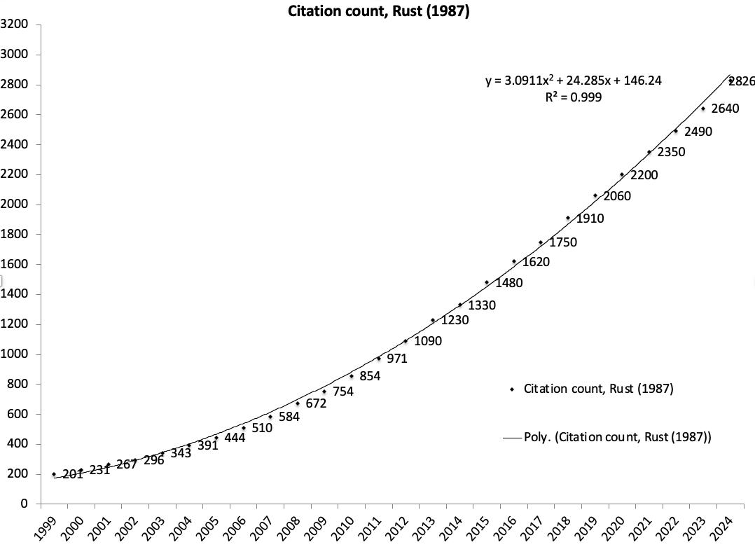
Dynamics of citation count of Rust (1987) Zurcher paper

📚 Who cares about Harold Zurcher?#

Occupational Choice (Keane and Wolpin, JPE 1997)
Retirement (Rust and Phelan, ECMA 1997)
Brand choice and advertising (Erdem and Keane, MaScience 1996)
Choice of college major (Arcidiacono, JoE 2004)
Individual migration decisions (Kennan and Walker, ECMA 2011)
High school attendance and work decisions (Eckstein and Wolpin, ECMA 1999)
Sales and dynamics of consumer inventory behavior (Hendel and Nevo, ECMA 2006)
Advertising, learning, and consumer choice in experience good markets (Ackerberg, IER 2003)
Route choice models (Fosgerau et al, Transp. Res. B)
Fertility and labor supply decisions (Francesconi, JoLE 2002)
Residential and Work-location choice (Buchinsky et al, ECMA 2015)
Equilibrium Allocations Under Alternative Waitlist Designs: Evidence From Deceased Donor Kidneys (Argarwal et al, ECMA 2021)
Equilibrium Trade in Automobiles (Gillingham, Iskhakov, Munk-Nielsen, Rus, Schjerning, JPE 2022)
…and many more

To this day NFXP is very powerful method for both solving and estimating dynamic discrete choice models

📖 Iskhakov et al. [2016] (Econometrica) “Comment on “Constrained Optimization Approaches to Estimation of Structural Models”” – we show that with proper implementation Rust’s method is as powerful as modern general solvers unleashed at the similar problem today

Components of the dynamic model#

State variables — vector of variables that describe all relevant information about the modeled decision process, \(x_t\)
Decision variables — vector of variables describing the choices, \(d_t\)
Instantaneous payoff — utility function, \(u(x_t,d_t)\), with time separable discounted utility
Motion rules — agent’s beliefs of how state variable evolve through time, conditional on choices, \(x_{t+1} \sim f(x_t,d_t)\)
Value function — maximum attainable utility \(V(x_t)\)
Policy function — mapping from state space to action space \(\delta : x_t \mapsto d^{\star}(x_t)\) that returns the optimal choice

Harold Zurcher engine replacement problem#

Harold Alois Zuercher
Superintendent of the Madison, Wisconsin bus company
June 16, 1926 - June 21, 2020

States and choices#

choice set: \(\{ \text{keep} , \text{replace} \} = \{0,1\}\)

Each bus comes in for repair once a month and Zurcher chooses between ordinary maintenance \((d_{t}=0)\) and overhaul/engine replacement \((d_{t}=1)\).

state space: mileage at time t since last engine overhaul \(x_t\)

Harold observes many different attributes of the buses which come into the shop, but we focus on the main one for now

Zurcher’s preferences#

Instantaneous payoffs are given by the cost function that depends on the choice

\[\begin{split}\begin{aligned} u(x_{t},d_t,\theta_1)=\left \{ \begin{array}{ll} -RC-c(0,\theta_1) & \text{if }d_{t}=\text{replace}=1 \\ -c(x_{t},\theta_1) & \text{if }d_{t}=\text{keep}=0 \end{array} \right. \end{aligned}\end{split}\]

\(RC\) = replacement cost
\(c(x,\theta_1)\) = cost of maintenance with preference parameters \(\theta_1\)

Motion rules#

First of all, mileage is continuous. How to deal with the continuous state space?
Rust discretized the range of travelled miles into \(n=175\) bins, indexed with \(i\), \(\hat{X} = \{\hat{x}_1,...,\hat{x}_n\}\) with \(\hat{x}_1=0\)

Mileage transition probability: for \(j = 0,...,J\)

\[\begin{split}\begin{aligned} p(x'|\hat{x}_k, d,\theta_2)= \begin{cases} Pr\{x'=\hat{x}_{k+j}|\theta_2\}= \theta_{2j} \text{ if } d=0 \\ Pr\{x'=\hat{x}_{1+j}|\theta_2\}= \theta_{2j} \text{ if } d=1 \end{cases} \end{aligned}\end{split}\]

Mileage in the next period \(x'\) can move up at most \(J\) grid points
\(J\) is determined from the observed distribution of mileage
Effectively, the probabilities of increase of mileage from any existing mileage are the same

If not replacing (\(d=0)\)

\[\begin{split}\begin{aligned} \Pi(d=0)_{n \times n} = \begin{pmatrix} \theta_{20} & \theta_{21} & \theta_{22} & 0 & \cdot & \cdot & \cdot & 0 \\ 0 & \theta_{20} & \theta_{21} & \theta_{22} & 0 & \cdot & \cdot & 0 \\ 0 & 0 &\theta_{20} & \theta_{21} & \theta_{22} & 0 & \cdot & 0 \\ \cdot & \cdot & \cdot & \cdot & \cdot & \cdot & \cdot & \cdot \\ 0 & \cdot & \cdot & 0 & \theta_{20} & \theta_{21} & \theta_{22} & 0 \\ 0 & \cdot & \cdot & \cdot & 0 & \theta_{20} & \theta_{21} & \theta_{22} \\ 0 & \cdot & \cdot & \cdot & \cdot & 0 & \theta_{20} & 1-\theta_{20} \\ 0 & \cdot & \cdot & \cdot & \cdot & \cdot & 0 & 1 \end{pmatrix} \end{aligned}\end{split}\]

If replacing (\(d=1)\)

\[\begin{split}\begin{aligned} \Pi(d=1)_{n \times n} = \begin{pmatrix} \theta_{20} & \theta_{21} & \theta_{22} & 0 & \cdot & \cdot & \cdot & 0 \\ \theta_{20} & \theta_{21} & \theta_{22} & 0 & \cdot & \cdot & \cdot & 0 \\ \theta_{20} & \theta_{21} & \theta_{22} & 0 & \cdot & \cdot & \cdot & 0 \\ \cdot & \cdot & \cdot & \cdot & \cdot & \cdot & \cdot & \cdot \\ \theta_{20} & \theta_{21} & \theta_{22} & 0 & \cdot & \cdot & \cdot & 0 \\ \theta_{20} & \theta_{21} & \theta_{22} & 0 & \cdot & \cdot & \cdot & 0 \\ \theta_{20} & \theta_{21} & \theta_{22} & 0 & \cdot & \cdot & \cdot & 0 \\ \end{pmatrix} \end{aligned}\end{split}\]

Dynamic optimization and Bellman equation#

To minimize the discounted expected value of the costs, Zurcher should find such policy function \(\delta(x_t):X\rightarrow \{\text{keep},\text{replace}\}\) such that \(d_t=\delta(x_t)\) maximizes

\[\mathbb{E}\sum_{t=0}^{\infty} \beta^t u(x_t,d_t) \longrightarrow \max\]

The function \(V(x_t)\) denotes the maximum attainable value at period t

\[V(x_t) = max_{\Pi} \mathbb{E} \sum_{j=t}^{\infty} \beta^{j-t} u(x_t,d_t)\]

where \(\Pi\) is a space of policy functions \(\delta(x_t):X\rightarrow \{\text{keep},\text{replace}\}\), and \(d_t = \delta(x_t)\)

Using Bellman Principle of Optimality, we can show that the value function \(V(x_t)\) constitutes the solution of the following functional equation

\[V(x) = \max_{d\in \{\text{keep},\text{replace}\}} \big\{ u(x,d) + \beta \mathbb{E}\big[ V(x')\big|x,d\big] \big\}\]

where expectation is taken over the next period values of state \(x'\) given the motion rule of the problem

Bellman operator#

The above Bellman equation can be written as a fixed point equation of the Bellman operator in the functional space

\[T(V)(x) \equiv \max_{d \in \{\text{keep},\text{replace}\}} \big\{ u(x,d) + \beta \mathbb{E}\big[ V(x') \big|x,d\big] \big\}\]

The Bellman equations is then \(V(x) = T(V)(x)\), with the solution given by the fixed point \(T(V) = V\)

Classification of the Zurcher model: Finite or infinite horizon? Discrete or continuous choice? Discrete or continuous states? Suitable solution methods?

Making the model suitable for empirical work#

Remember that Zurcher observes many different attributes of the busses that come into the shop
But we as an econometrician do not!
Yet, these are likely to be the reason for observing different behavior in same states (for the same observed mileage)

Need to include error terms into the model, denote \(\epsilon\)

Back to the RUM framework of \(u(d,x)+\epsilon(d)\) but now in dynamic setting

Should the error term be part of the state space of the problem?

Updating the Bellman equation#

\(\varepsilon\) is a new (vector) state variable

\[V(x,\varepsilon) = \max_{d\in \{0,1\}} \big\{ u(x,\varepsilon_d,d) + \beta \mathbb{E}\big[ V(x',\varepsilon')\big|x,\varepsilon,d\big] \big\}\]

\[V(x,\varepsilon) = \max_{d\in \{0,1\}} \big\{ u(x,\varepsilon_d,d) + \beta \int_{X} \int_{\Omega} V(x',\varepsilon') p(x',\varepsilon'|x,\varepsilon,d) dx'd\varepsilon' \big\}\]

where \(\varepsilon_d\) is the component of vector \(\varepsilon \in \mathbb{R}^2\) which corresponds to \(d\)

Rust assumptions#

(AS) Additive separability in preferences

\[u(x,\varepsilon_d,d) = u(x,d) + \varepsilon_d,\]

same as in the static RUM models

(CI) Conditional independence

\[p(x',\varepsilon'|x,\varepsilon,d) = q(\varepsilon'|x')\cdot \pi(x'|x,d)\]

in addition to standard independence assumptions of static RUM
1. Error terms are independent across observations due to random sampling
2. Error terms come as vectors, one for each decision, and are independent across choices
And additional assumption for dynamic models: conditional on \(x\), there is no serial correlation in error terms across time

(EV) Extreme value Type I (EV1) distribution of \(\varepsilon\)

making things simpler by providing closed form expressions for choice probabilities
can be easily relaxed to GEV, and with the trouble of multidimensional integration to other continuous distribution with full support

What Rust assumptions allow:#

\[V(x,\varepsilon) = \max_{d\in \{0,1\}} \big\{ u(x,d) + \varepsilon_d + \beta \int_{X} \int_{\Omega} V(x',\varepsilon') \pi(x'|x,d) q(\varepsilon'|x') dx' d\varepsilon' \big\}\]

Separate out the deterministic part of choice specific value function \(v(x,d)\) (SA)
Compute the expectation by part (CI)
Use max-stability of EV1 to compute expectation w.r.t. \(\varepsilon'\) (EV)

\[V(x,\varepsilon) = \max_{d\in \{0,1\}} \big\{ \underbrace{u(x,d) + \beta \int_{X} \Big( \int_{\Omega} V(x',\varepsilon') q(\varepsilon'|x') d\varepsilon'\Big) \pi(x'|x,d) dx'}_{v(x,d)} + \varepsilon_d \big\}\]

\[V(x',\varepsilon') = \max_{d\in \{0,1\}} \big\{ v(x',d) + \varepsilon'_d \big\}\]

\[\mathbb{E}\big[ V(x',\varepsilon')\big|x,d\big] = \int_{X} \log \big( \exp[v(x',0)] + \exp[v(x',1)] \big) \pi(x'|x,d) dx'\]

Bellman equation and Bellman operator in expected value function space#

Let \(\mathbb{E}\big[ V(x',\varepsilon')\big|x,d\big] = EV(x,d)\), then

\[\begin{split}\begin{aligned} \begin{eqnarray} EV(x,d) &=& \int_{X} \log \big( \exp[v(x',0)] + \exp[v(x',1)] \big) \pi(x'|x,d) dx' \\ v(x,d) &=& u(x,d) + \beta EV(x,d) \end{eqnarray} \end{aligned}\end{split}\]

this is Bellman equation in expected value function space
when the state space is discrete the integral is, of course, a simple sum over future values

Writing all together we have

\[EV(x,d) = \sum_{X} \log \big( \exp[u(x',0) + \beta EV(x',0)] + \exp[u(x',1) + \beta EV(x',1)] \big) \pi(x'|x,d)\]

and can define the operator \(T^*\) in the expected value function space

\[T^*(EV)(x,d) \equiv \sum_{X} \log \big( \exp[u(x',0) + \beta EV(x',0)] + \exp[u(x',1) + \beta EV(x',1)] \big) \pi(x'|x,d)\]

Solution to the Bellman functional equation \(EV(x,d)\) is also a fixed point of \(T^*\) operator, \(T^*(EV)(x,d)=EV(x,d)\)

\(T^*\) is also a contraction mapping in the space of expected value functions as shown by Ma and Stachurski [2021]
Contraction mapping \(\Rightarrow\) VFI is guaranteed to find the unique solution!
Dimentionality of this fixed point problem is smaller that the one in value function terms (because \(\varepsilon\) is not included)
It is also numerically easier to work with smooth expected values \(EV(x,d)\) rather than \(V(x,\varepsilon)\)
Later we’ll also see a very nice numerical optimization possibilities as well

Choice probabilities#

Once the fixed point is found, the optimal choice probability \(P(d|x)\) is given by the Logit structure (assumption EV):

\[P(d|x) = \frac{\exp[v(x,d)]}{\sum_{d'\in \{0,1\}} \exp[v(x,d')]}\]

The choice probability serve as the bases for forming the likelihood function. Will continue with this when talking about structural estimation!

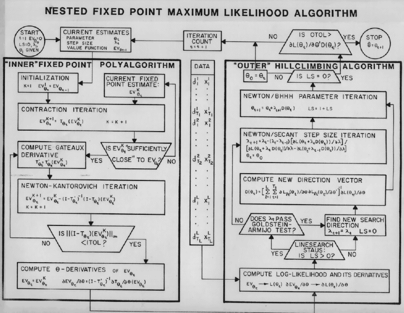
NK iterations method#

Zurcher model has the following features:

infinite horizon
discretized mileage which is the only state (in EV formulation) = finite state space
discrete choice
idiosyncratic random components

Therefore the suitable solution methods are

value function iterations (VFI)
policy iterations video 43 in CompEcon course
Newton-Kantorovich method (NK iterations)

application of Newton method in functional spaces
numerically equivalent to policy iterations

\[EV(x,d) = T^*(EV)(x,d) = \Gamma(EV)(x,d) \quad\Leftrightarrow\quad (I - \Gamma)(EV)(x,d)=\mathbb{0}\]

The NK iteration is

\[EV_{k+1} = EV_{k} - (I-\Gamma')^{-1} (I-\Gamma)(EV_k)\]

The new operator is the difference between the identity operator \(I\) and Bellman operator \(\Gamma = T^*\)
\(\mathbb{0}\) is zero function
\(I-\Gamma'\) is a Fréchet derivative of the operator \(I-\Gamma\)

We work with finite approximations on the discrete state space \(\rightarrow\) vectors and matrixes!

let \(n\) denote the number of state points (in mileage)
\(EV(x,d)\) is given by a vector of length \(n\), assuming that the first element is reused to describe the expected value of replacing
\(T^*(EV)(x,d) = \Gamma(EV)(x,d)\) is a non-linear \(n\)-valued multivariate function of \(EV\)
Fréchet derivative \(I-\Gamma'\) is an \(n \times n\) matrix of first order derivatives of each output of \(T^*(EV)(x,d)\) w.r.t. each input

Therefore: NK iterations on finite approximations are similar to solving a system of \(n\) equations with \(n\) unknowns with Newton method!

Matrix expression for the finite approximation of the Bellman operator#

\[EV(x,d) = \sum_{X} \log \big( \exp[u(x',0) + \beta EV(x',0)] + \exp[u(x',1) + \beta EV(x',1)] \big) \pi(x'|x,d)\]

\[EV = \Pi \cdot L \big( U(\text{keep}) + \beta EV, U(\text{replace}) + \beta EV[0] \big)\]

\(EV\) is a \(n \times 1\) column vector
\(\Pi\) is the \(n \times n\) matrix of mileage transition probabilities
\(U(\cdot)\) is a column-vector of costs for all points in the state space, conditional on decision
\(L(\cdot,\cdot)\) is the logsum function returning an \(n \times 1\) vector
notation \(\bullet[i]\) denotes the \(i\)-th element a vector

Implementation of Fréchet derivative#

Finite approximation of the Bellman operator is

\[\Gamma(EV) = \Pi \cdot L \big( U(\text{keep}) + \beta EV, U(\text{replace}) + \beta EV[0] \big)\]

Fréchet derivative w.r.t. \(EV\) is then given by \(n \times n\) matrix

\[\frac{\partial \Gamma}{\partial EV} = \Pi \cdot \frac{\partial L\big( U(\text{keep}) + \beta EV, U(\text{replace}) + \beta EV[0] \big)}{\partial EV}\]

Differentiating the logsum function w.r.t. a scalar#

the logsum function \(L(w_1,w_2) = \log\big[ \exp(w_1) + \exp(w_2) \big]\)
(\(L(w_1,w_2)\) is the expectation of maximum of \(w_i + \varepsilon_i\), where \(\varepsilon_1, \varepsilon_2\) are distributed independently with type 1 extreme value distribution)
let \(p_i = {\exp(w_i) \over \exp(w_1) + \exp(w_2)}\) denote the corresponding choice probabilities

\[\frac{\partial L(w_1,w_2)}{\partial x} = p_1 \frac{\partial w_1}{\partial x} + p_2 \frac{\partial w_2}{\partial x}\]

Differentiating the logsum function w.r.t. \(EV[i],\;i>0\)#

\[\begin{split}\begin{aligned} \frac{\partial L}{\partial EV} = \beta \begin{pmatrix} \bullet & 0 & 0 & 0 & \cdot & 0 \\ \bullet & P[1] & 0 & 0 & \cdot & 0 \\ \bullet & 0 & P[2] & 0 & \cdot & 0 \\ \bullet & 0 & 0 & P[3] & \cdot & 0 \\ \cdot & \cdot & \cdot & \cdot & \cdot & \cdot \\ \bullet & 0 & 0 & 0 & \cdot & P[n-1] \end{pmatrix} \end{aligned}\end{split}\]

where \(P[i]\) is a shortcut notation for probability of keeping \(P(0|x[i])\) at state point \(i\)

Differentiating the logsum function w.r.t. \(EV[0]\)#

\[\begin{split}\begin{aligned} \frac{\partial L}{\partial EV[0]} = \beta \begin{pmatrix} P[0] + \bar{P}[0] \\ \bar{P}[1] \\ \bar{P}[2] \\ \cdot \\ \bar{P}[n-1] \end{pmatrix} \end{aligned}\end{split}\]

where \(\bar{P}[i]\) is a shortcut notation for probability of replacing \(P(1|x[i])\) at state point \(i\)

Matrix notation for the Fréchet derivative#

\[\begin{split}\begin{aligned} \frac{\partial \Gamma}{\partial EV} = \beta \begin{pmatrix} \theta_{20} & \theta_{21} & \theta_{22} & 0 & \cdot & \cdot & \cdot & 0 \\ 0 & \theta_{20} & \theta_{21} & \theta_{22} & 0 & \cdot & \cdot & 0 \\ \cdot & \cdot & \cdot & \cdot & \cdot & \cdot & \cdot & \cdot \\ 0 & \cdot & \cdot & \cdot & 0 & \theta_{20} & \theta_{21} & \theta_{22} \\ 0 & \cdot & \cdot & \cdot & \cdot & 0 & \theta_{20} & 1-\theta_{20} \\ 0 & \cdot & \cdot & \cdot & \cdot & \cdot & 0 & 1 \end{pmatrix} \begin{pmatrix} P[0] + \bar{P}[0] & 0 & 0 & 0 & \cdot & 0 \\ \bar{P}[1] & P[1] & 0 & 0 & \cdot & 0 \\ \bar{P}[2] & 0 & P[2] & 0 & \cdot & 0 \\ \bar{P}[3] & 0 & 0 & P[3] & \cdot & 0 \\ \cdot & \cdot & \cdot & \cdot & \cdot & \cdot \\ \bar{P}[n-1] & 0 & 0 & 0 & \cdot & P[n-1] \end{pmatrix} \end{aligned}\end{split}\]

Matrix notation for the Fréchet derivative#

\[\begin{split}\begin{aligned} \frac{\partial \Gamma}{\partial EV} = \beta \begin{pmatrix} \theta_{20} P[0] & \theta_{21} P[1] & \theta_{22} P[2] & 0 & \cdot & \cdot & \cdot & 0 \\ 0 & \theta_{20}P[1] & \theta_{21}P[2] & \theta_{22}P[3] & 0 & \cdot & \cdot & 0 \\ 0 & 0 &\theta_{20}P[2] & \theta_{21}P[3] & \theta_{22}P[4] & 0 & \cdot & 0 \\ \cdot & \cdot & \cdot & \cdot & \cdot & \cdot & \cdot & \cdot \\ \cdot & \cdot & \cdot & \cdot & \cdot & \cdot & 0 & P[n-1] \end{pmatrix} + \beta \begin{pmatrix} \Pi \bar{P}, 0, \dots, 0 \end{pmatrix} \end{aligned}\end{split}\]

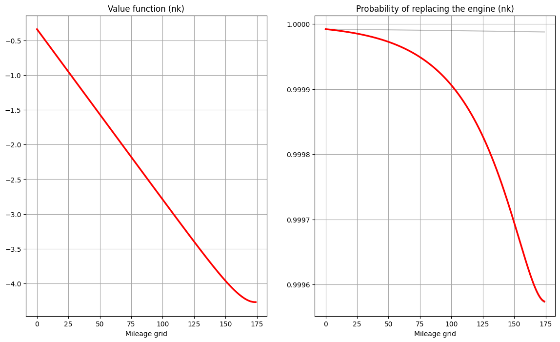
NK iterations algorithm#

Initialize value function at \(EV_0\) (starting values matter!)
Perform the Newton-Kantorovich step, computing the policy function along the way of applying the Bellman operator \(\Gamma(\cdot)\)

\[EV_{k+1} = EV_{k} - (I-\Gamma')^{-1} (I-\Gamma)(EV_k)\]

Repeat until convergence value function space

import numpy as np
import matplotlib.pyplot as plt
%matplotlib inline

class zurcher():
    '''Harold Zurcher bus engine replacement model class, VFI version'''

    def __init__(self,
                 n = 175,           # number of state points
                 RC = 11.7257,      # replacement cost
                 c = 2.45569,       # parameter of maintance cost (theta_1)
                 p = [0.0937,0.4475,0.4459,0.0127],  # probabilities of transitions (theta_2)
                 beta = 0.9999):    # discount factor
        '''Init for the Zurcher model object'''
        assert sum(p)<=1.0, 'Transition probability parameters must sum up to <1'
        self.RC, self.c, self.p, self.beta, self.n= RC, c, p, beta, n

    @property
    def n(self):
        '''Attrinute getter for n'''
        return self.__n

    @n.setter
    def n(self, value):
        '''Attribute n setter'''
        self.__n = value
        self.grid = np.arange(self.__n)
        self.trpr = self.__transition_probs()

    def __repr__(self):
        '''String representation of the Zurcher model'''
        return 'Rust model of bus engine replacement (id={})'.format(id(self))

    def __transition_probs(self):
        '''Computing the transision probability matrix'''
        trpr = np.zeros((self.__n,self.__n))  # init
        probs = self.p + [1-sum(self.p)]  # ensure sum up to 1
        for i,p in enumerate(probs):
            trpr += np.diag([p]*(self.__n-i),k=i)
        trpr[:,-1] = 1.-np.sum(trpr[:,:-1],axis=1) 
        return trpr

    def bellman(self,ev0,deriv=False):
        '''Bellman operator for the model
           Depending on deriv argument, returns 2 or 3 outputs (Fréchet derivative)
        '''
        x = self.grid  # points in the next period state
        mcost = -0.001*x*self.c                         # 1-dim array of maintenance costs 
        vx0 = mcost + self.beta * ev0                   # 1-dim array v(x,0), keep
        vx1 = mcost[0] - self.RC + self.beta * ev0[0]   # 1-dim array v(x,1), replace
        M = np.maximum(vx0,vx1)                         # de-max values to avoid exp(large number)
        logsum = M + np.log(np.exp(vx0-M) + np.exp(vx1-M))
        ev1 = self.trpr @ logsum                        # 1-dim array after matrix multiplication
        pk = 1/( np.exp(vx1-vx0)+1 )                    # choice prob to keep
        if not deriv:
            return ev1, pk
        # Fréchet derivative
        dev1 = self.beta * self.trpr * pk[np.newaxis,:] # element-wise, pk in rows
        dev1[:,0] += self.beta * self.trpr @ (1-pk)     # w.r.t. EV[0] special case
        return ev1, pk, dev1

    def solve_vfi(self,tol=1e-6,maxiter=100,callback=None):
        '''Solves the Rust model using value function iterations
        '''
        ev0 = np.zeros(self.n) # initial point for VFI
        err0 = 1.0 # initial lagged error
        for iter in range(maxiter):  # main loop
            ev1, pk = self.bellman(ev0)  # update approximation
            err = np.amax(np.abs(ev0-ev1))
            if callback:
                callback(iter=iter,model=self,ev1=ev1,ev0=ev0,err=err,err_prev=err0,pk=pk,method='vfi',itertype='sa')
            if err<tol:
                break  # break out if converged
            ev0 = ev1  # get ready to the next iteration
            err0 = err
        else:
            raise RuntimeError('Failed to converge in %d iterations'%maxiter)
        return ev1, pk

    def solve_nk(self, maxiter=100, tol=1e-6, callback=None):
        '''Solves the model using the Newton-Kantorovich iterations
        '''
        ev0 = np.zeros(self.n) # initial point
        err0 = 1.0 # initial lagged error
        for iter in range(maxiter):
            ev1,pk,dev = self.bellman(ev0,deriv=True) # compute with Fréchet derivative
            ev1 = ev0 - np.linalg.solve(np.eye(self.n)-dev,ev0 - ev1)  # NK step
            err = np.max(np.abs(ev1-ev0))
            if callback:
                callback(iter=iter,model=self,ev1=ev1,ev0=ev0,err=err,err_prev=err0,pk=pk,method='nk',itertype='nk')
            if err < tol: 
                break  # break out if converged
            ev0 = ev1  # get ready to the next iteration
            err0 = err
        else:
            raise RuntimeError('Failed to converge in %d iterations'%maxiter)
        ev1,pk = self.bellman(ev1) # compute choice probabilities after convergence
        return ev1,pk

    def solve_poly(self, 
                   maxiter=100, 
                   tol=1e-10, 
                   sa_min=5,         # minimum number of contraction steps
                   sa_max=25,        # maximum number of contraction steps
                   switch_tol=0.025, # tolerance of the switching rule
                   callback=None):
        '''Solves the model using the poly-algorithm'''
        ev0 = np.zeros(self.n) # initial point
        err0 = 1.0 # initial lagged error
        nk = False # start with successive approximations
        for iter in range(maxiter):
            ev1,pk,dev = self.bellman(ev0,deriv=True) # update EV for both types of a step
            err = np.max(np.abs(ev1-ev0))
            nk = True if iter>= sa_max else nk  # have to switch to NK after sa_max
            nk = nk or (iter>=sa_min and abs(err/err0 - self.beta)<switch_tol)  # check if need to switch to NK
            if nk:
                ev1 = ev0 - np.linalg.solve(np.eye(self.n)-dev,ev0 - ev1)  # NK step
                err = np.max(np.abs(ev1-ev0))
            if callback:
                itertype = 'nk' if nk else 'sa'  # label for the iteration type
                callback(iter=iter,model=self,ev1=ev1,ev0=ev0,err=err,err_prev=err0,pk=pk,method='poly',itertype=itertype)
            if err < tol: 
                break  # break out if converged
            ev0 = ev1  # get ready to the next iteration
            err0 = err
        else:
            raise RuntimeError('No convergence: maximum number of iterations achieved! Increase maxiter')
        ev1,pk = self.bellman(ev1) # compute choice probabilities after convergence
        return ev1,pk

    def solve_show(self,solver='vfi',verbosity=0,plot=True,**kvargs):
        '''Illustrate solution for given solver = {vfi,nk,poly} and 
           print errors/relative errors from iterations (when verbose=True)
           All other arguments are passed to the solver
        '''
        if solver=='vfi':
            chosen_solver = self.solve_vfi
        elif solver=='nk':
            chosen_solver = self.solve_nk
        elif solver=='poly':
            chosen_solver = self.solve_poly
        else:
            raise RuntimeError('Unknown solver in solve_show()')
        if plot:
            fig1, (ax1,ax2) = plt.subplots(1,2,figsize=(14,8))
            ax1.grid(visible=True, which='both', color='0.65', linestyle='-')
            ax2.grid(visible=True, which='both', color='0.65', linestyle='-')
            ax1.set_xlabel('Mileage grid')
            ax2.set_xlabel('Mileage grid')
            ax1.set_title(f'Value function ({solver})')
            ax2.set_title(f'Probability of replacing the engine ({solver})')
        def callback(**argvars):
            iter,itertype,err,derr = argvars['iter'],argvars['itertype'],argvars['err'],argvars['err_prev']
            mod, ev, pk = argvars['model'],argvars['ev1'],argvars['pk']
            if verbosity>1:
                if iter==0:
                    print('Solver = %s'%solver)
                    print('-'*42)
                    print('%7s %16s %16s'%('iter','err','err(i)/err(i-1)'))
                    print('-'*42)
                print('%4d %2s %16.4e %16.12f'%(iter,itertype[:2],err,err/derr))
            elif verbosity>0:
                if iter==0:
                    print('Solver = %s'%solver)
                    print('-'*22)
                    print('%4s %16s'%('iter','err'))
                    print('-'*22)
                print('%4d %16.4e'%(iter,err))
            if plot:
                ax1.plot(mod.grid,ev,color='k',alpha=0.25)
                ax2.plot(mod.grid,pk,color='k',alpha=0.25)
            callback.nriter = iter  # save iter in function object attribute
        # run the chosen solver
        ev,pk = chosen_solver(callback=callback,**kvargs)
        if plot:
            # add solutions
            ax1.plot(self.grid,ev,color='r',linewidth=2.5)
            ax2.plot(self.grid,pk,color='r',linewidth=2.5)
            plt.show()
        print('{} solved with {} in {} iterations'.format(self,solver,callback.nriter))
        return ev,pk    

# compare SA, NK
model = zurcher(beta=0.9)  # try different value of beta
ev1,pk1 = model.solve_show(maxiter=1500)
ev2,pk2 = model.solve_show(solver='nk')
print()
print('Max diff between value functions is ' ,np.amax(np.abs(ev1-ev2)))
print('Max diff between policy functions is',np.amax(np.abs(pk1-pk2)))

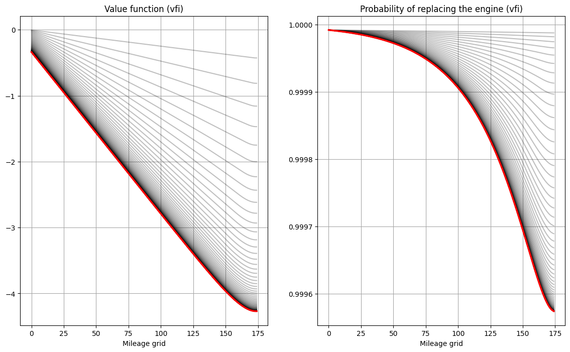
_images/d9b268a4ff0f294d4f7995e4471bab26cc1417f6064eb6af337df4085a18e46a.png

Rust model of bus engine replacement (id=140079555197968) solved with vfi in 123 iterations

_images/717092d3916875932d96200085e3e8dab205c88fff95a274e99165a4c9b89cf9.png

Rust model of bus engine replacement (id=140079555197968) solved with nk in 2 iterations

Max diff between value functions is  8.957091488293045e-06
Max diff between policy functions is 9.113154675333135e-12

Does VFI algorithm always converge? What determines the speed of convergence of the VFI algorithm? Does NK algorithm always converge?

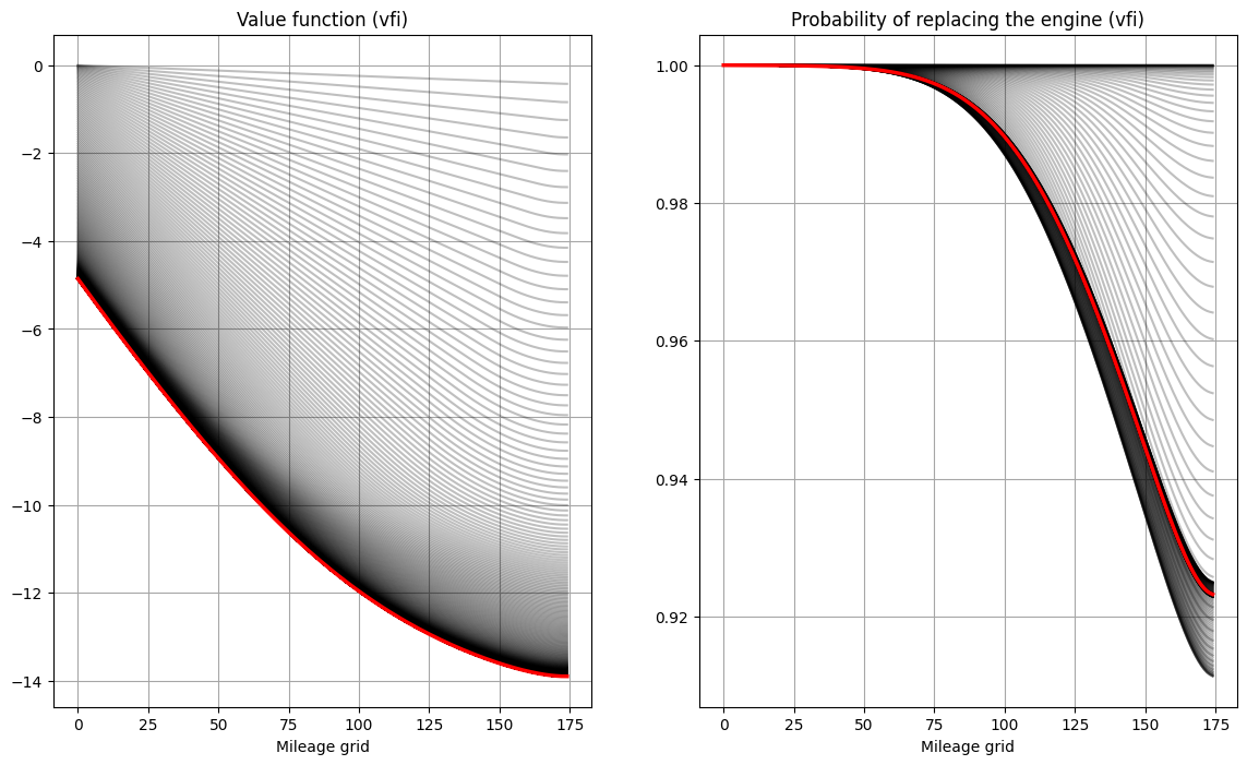
Properties of VFI vs Newton-Kantorovich solution methods#

VFI is globally convergent (Bellman is contraction mappint \(\Rightarrow\) single fixed point)
VFI convergent rate is \(beta\), very slow in approaching the fixed point when \(beta\) is close to one

vs.

Newton-Kantorovich has quadratic convergence rate
Newton-Kantorovich is sensitive to starting point

# compare SA, NK
model = zurcher(beta=0.975)
ev1,pk1 = model.solve_show(maxiter=1500,verbosity=1,plot=False)
ev2,pk2 = model.solve_show(solver='nk',verbosity=1,plot=False)
print()
print('Max diff between value functions is ' ,np.amax(np.abs(ev1-ev2)))
print('Max diff between policy functions is',np.amax(np.abs(pk1-pk2)))

Solver = vfi
----------------------
iter              err
----------------------
     4.2728e-01
     4.1659e-01
     4.0617e-01
     3.9600e-01
     3.8608e-01
     3.7640e-01
     3.6696e-01
     3.5773e-01
     3.4873e-01
     3.3992e-01
     3.3131e-01
     3.2289e-01
     3.1464e-01
     3.0655e-01
     2.9862e-01
     2.9082e-01
     2.8316e-01
     2.7562e-01
     2.6820e-01
     2.6088e-01
     2.5366e-01
     2.4654e-01
     2.3952e-01
     2.3258e-01
     2.2576e-01
     2.1904e-01
     2.1242e-01
     2.0592e-01
     1.9954e-01
     1.9331e-01
     1.8722e-01
     1.8127e-01
     1.7549e-01
     1.6987e-01
     1.6443e-01
     1.5916e-01
     1.5408e-01
     1.4919e-01
     1.4448e-01
     1.3995e-01
     1.3560e-01
     1.3143e-01
     1.2743e-01
     1.2360e-01
     1.1992e-01
     1.1639e-01
     1.1300e-01
     1.0975e-01
     1.0662e-01
     1.0361e-01
     1.0072e-01
     9.7925e-02
     9.5235e-02
     9.2641e-02
     9.0134e-02
     8.7710e-02
     8.5366e-02
     8.3101e-02
     8.0904e-02
     7.8777e-02
     7.6716e-02
     7.4714e-02
     7.2777e-02
     7.0891e-02
     6.9065e-02
     6.7287e-02
     6.5563e-02
     6.3884e-02
     6.2255e-02
     6.0666e-02
     5.9125e-02
     5.7622e-02
     5.6162e-02
     5.4739e-02
     5.3355e-02
     5.2007e-02
     5.0692e-02
     4.9415e-02
     4.8168e-02
     4.6956e-02
     4.5773e-02
     4.4621e-02
     4.3499e-02
     4.2404e-02
     4.1339e-02
     4.0300e-02
     3.9287e-02
     3.8302e-02
     3.7338e-02
     3.6402e-02
     3.5488e-02
     3.4596e-02
     3.3729e-02
     3.2882e-02
     3.2057e-02
     3.1253e-02
     3.0468e-02
     2.9704e-02
     2.8958e-02
     2.8232e-02
     2.7524e-02
     2.6832e-02
     2.6160e-02
     2.5504e-02
     2.4864e-02
     2.4241e-02
     2.3632e-02
     2.3040e-02
     2.2461e-02
     2.1898e-02
     2.1349e-02
     2.0813e-02
     2.0291e-02
     1.9782e-02
     1.9276e-02
     1.8768e-02
     1.8258e-02
     1.7745e-02
     1.7229e-02
     1.6711e-02
     1.6191e-02
     1.5669e-02
     1.5172e-02
     1.4790e-02
     1.4409e-02
     1.4027e-02
     1.3648e-02
     1.3272e-02
     1.2902e-02
     1.2538e-02
     1.2183e-02
     1.1836e-02
     1.1498e-02
     1.1171e-02
     1.0854e-02
     1.0546e-02
     1.0249e-02
     9.9619e-03
     9.6842e-03
     9.4159e-03
     9.1565e-03
     8.9057e-03
     8.6634e-03
     8.4290e-03
     8.2021e-03
     7.9827e-03
     7.7703e-03
     7.5645e-03
     7.3651e-03
     7.1718e-03
     6.9844e-03
     6.8026e-03
     6.6262e-03
     6.4550e-03
     6.2886e-03
     6.1270e-03
     5.9700e-03
     5.8173e-03
     5.6690e-03
     5.5246e-03
     5.3843e-03
     5.2477e-03
     5.1147e-03
     4.9853e-03
     4.8594e-03
     4.7367e-03
     4.6173e-03
     4.5009e-03
     4.3877e-03
     4.2772e-03
     4.1697e-03
     4.0650e-03
     3.9629e-03
     3.8634e-03
     3.7664e-03
     3.6720e-03
     3.5798e-03
     3.4901e-03
     3.4026e-03
     3.3173e-03
     3.2342e-03
     3.1532e-03
     3.0742e-03
     2.9972e-03
     2.9221e-03
     2.8489e-03
     2.7776e-03
     2.7080e-03
     2.6402e-03
     2.5741e-03
     2.5096e-03
     2.4468e-03
     2.3855e-03
     2.3258e-03
     2.2676e-03
     2.2108e-03
     2.1555e-03
     2.1015e-03
     2.0489e-03
     1.9976e-03
     1.9475e-03
     1.8988e-03
     1.8513e-03
     1.8049e-03
     1.7598e-03

     1.7157e-03
     1.6727e-03
     1.6309e-03
     1.5900e-03
     1.5498e-03
     1.5101e-03
     1.4710e-03
     1.4325e-03
     1.3946e-03
     1.3573e-03
     1.3207e-03
     1.2847e-03
     1.2493e-03
     1.2147e-03
     1.1814e-03
     1.1518e-03
     1.1227e-03
     1.0941e-03
     1.0660e-03
     1.0384e-03
     1.0114e-03
     9.8509e-04
     9.5936e-04
     9.3426e-04
     9.0979e-04
     8.8595e-04
     8.6275e-04
     8.4016e-04
     8.1818e-04
     7.9681e-04
     7.7602e-04
     7.5580e-04
     7.3614e-04
     7.1703e-04
     6.9845e-04
     6.8038e-04
     6.6281e-04
     6.4573e-04
     6.2911e-04
     6.1296e-04
     5.9724e-04
     5.8196e-04
     5.6709e-04
     5.5262e-04
     5.3854e-04
     5.2485e-04
     5.1151e-04
     4.9853e-04
     4.8590e-04
     4.7360e-04
     4.6163e-04
     4.4997e-04
     4.3861e-04
     4.2755e-04
     4.1678e-04
     4.0628e-04
     3.9606e-04
     3.8610e-04
     3.7640e-04
     3.6694e-04
     3.5773e-04
     3.4875e-04
     3.4000e-04
     3.3147e-04
     3.2316e-04
     3.1506e-04
     3.0717e-04
     2.9947e-04
     2.9197e-04
     2.8466e-04
     2.7753e-04
     2.7058e-04
     2.6381e-04
     2.5720e-04
     2.5077e-04
     2.4449e-04
     2.3837e-04
     2.3241e-04
     2.2659e-04
     2.2092e-04
     2.1539e-04
     2.1001e-04
     2.0475e-04
     1.9963e-04
     1.9463e-04
     1.8976e-04
     1.8502e-04
     1.8039e-04
     1.7588e-04
     1.7148e-04
     1.6719e-04
     1.6300e-04
     1.5893e-04
     1.5495e-04
     1.5107e-04
     1.4729e-04
     1.4361e-04
     1.4002e-04
     1.3651e-04
     1.3310e-04
     1.2977e-04
     1.2652e-04
     1.2336e-04
     1.2027e-04
     1.1725e-04
     1.1429e-04
     1.1139e-04
     1.0855e-04
     1.0576e-04
     1.0304e-04
     1.0038e-04
     9.7771e-05
     9.5223e-05
     9.2731e-05
     9.0297e-05
     8.8017e-05
     8.5809e-05
     8.3648e-05
     8.1535e-05
     7.9470e-05
     7.7452e-05
     7.5482e-05
     7.3560e-05
     7.1686e-05
     6.9858e-05
     6.8077e-05
     6.6341e-05
     6.4649e-05
     6.3001e-05
     6.1396e-05
     5.9833e-05
     5.8310e-05
     5.6828e-05
     5.5384e-05
     5.3977e-05
     5.2608e-05
     5.1274e-05
     4.9975e-05
     4.8710e-05
     4.7478e-05
     4.6278e-05
     4.5109e-05
     4.3971e-05
     4.2862e-05
     4.1781e-05
     4.0729e-05
     3.9703e-05
     3.8704e-05
     3.7731e-05
     3.6783e-05
     3.5858e-05
     3.4958e-05
     3.4080e-05
     3.3225e-05
     3.2391e-05
     3.1579e-05
     3.0787e-05
     3.0015e-05
     2.9263e-05
     2.8530e-05
     2.7815e-05
     2.7119e-05
     2.6440e-05
     2.5778e-05
     2.5132e-05
     2.4503e-05
     2.3890e-05
     2.3292e-05
     2.2709e-05
     2.2141e-05
     2.1587e-05
     2.1047e-05
     2.0521e-05
     2.0007e-05
     1.9507e-05
     1.9019e-05
     1.8543e-05
     1.8080e-05
     1.7627e-05
     1.7187e-05
     1.6757e-05
     1.6338e-05
     1.5929e-05
     1.5531e-05
     1.5142e-05
     1.4764e-05
     1.4394e-05
     1.4034e-05
     1.3684e-05
     1.3341e-05
     1.3008e-05
     1.2682e-05
     1.2365e-05
     1.2056e-05
     1.1755e-05
     1.1461e-05
     1.1174e-05
     1.0895e-05
     1.0622e-05
     1.0357e-05
     1.0098e-05
     9.8451e-06
     9.5988e-06
     9.3588e-06
     9.1248e-06
     8.8962e-06
     8.6729e-06
     8.4547e-06
     8.2416e-06
     8.0334e-06
     7.8301e-06
     7.6316e-06
     7.4378e-06
     7.2486e-06
     7.0639e-06
     6.8837e-06
     6.7106e-06
     6.5426e-06
     6.3786e-06
     6.2185e-06
     6.0622e-06
     5.9097e-06
     5.7609e-06
     5.6158e-06
     5.4743e-06
     5.3363e-06
     5.2018e-06
     5.0707e-06
     4.9429e-06
     4.8183e-06
     4.6969e-06
     4.5786e-06
     4.4633e-06
     4.3509e-06
     4.2414e-06
     4.1347e-06
     4.0307e-06
     3.9294e-06
     3.8306e-06
     3.7344e-06
     3.6406e-06
     3.5491e-06
     3.4600e-06
     3.3732e-06
     3.2886e-06
     3.2061e-06
     3.1257e-06
     3.0473e-06
     2.9709e-06
     2.8965e-06
     2.8239e-06
     2.7531e-06
     2.6842e-06
     2.6170e-06
     2.5514e-06
     2.4876e-06
     2.4253e-06
     2.3646e-06
     2.3054e-06
     2.2477e-06
     2.1915e-06
     2.1366e-06
     2.0832e-06
     2.0311e-06
     1.9803e-06
     1.9307e-06
     1.8824e-06
     1.8354e-06
     1.7895e-06
     1.7447e-06
     1.7011e-06
     1.6585e-06
     1.6171e-06
     1.5766e-06
     1.5372e-06
     1.4988e-06
     1.4613e-06
     1.4247e-06
     1.3891e-06
     1.3544e-06
     1.3205e-06
     1.2875e-06
     1.2553e-06
     1.2239e-06
     1.1933e-06
     1.1635e-06
     1.1344e-06
     1.1060e-06
     1.0784e-06
     1.0514e-06
     1.0251e-06
     9.9949e-07
Rust model of bus engine replacement (id=140078659975376) solved with vfi in 496 iterations
Solver = nk
----------------------
iter              err
----------------------
     1.7085e+01
     1.6466e+00
     1.0015e+00
     4.7225e-01
     8.3180e-02
     2.1647e-03
     1.4257e-06
     6.1817e-13
Rust model of bus engine replacement (id=140078659975376) solved with nk in 7 iterations

Max diff between value functions is  3.884109376883771e-05
Max diff between policy functions is 2.4160655698324263e-09

Poly-algorithm#

NK method may not be convergent at the initial point
Successive apprizimataion (SA) iterations, however, are always convergent

Poly algorithm is combination of SA and NK:

Start with SA iterations
At approximately optimal time switch to NK iterations

When to switch to NK iterations?#

Suppose \(EV_{k-1} = {EV}^\star + C\) (where \({EV}^\star\) is the fixed point)

\[err_{k} = ||EV_{k-1}-EV_{k}|| = ||{EV}^\star+C - T^*({EV}^\star+C)|| = ||{EV}^\star + C - {EV}^\star - \beta C|| = C (1-\beta)\]

\[err_{k+1} = ||EV_{k}-EV_{k+1}|| = ||T^*({EV}^\star+C) - T^*(T^*({EV}^\star+C))|| = ||{EV}^\star + \beta C - {EV}^\star - \beta^2 C|| = \beta C (1-\beta)\]

Then the ration of two errors \(\frac{err_{k+1}}{err_{k}} = \beta\) when the current approximation is a constant away from the fixed point.
NK iteration will immediately “strip away” the constant

Thus, switch to NK iteration when \(\frac{err_{k+1}}{err_{k}}\) is close to \(\beta\)

# when to switch from SA to NK
model = zurcher(beta=0.975)
model.solve_show(maxiter=1500,verbosity=2,plot=False);

Solver = vfi
------------------------------------------
   iter              err  err(i)/err(i-1)
------------------------------------------
sa       4.2728e-01   0.427277667463
sa       4.1659e-01   0.974985156037
sa       4.0617e-01   0.974977898685
sa       3.9600e-01   0.974967530759
sa       3.8608e-01   0.974952914413
sa       3.7640e-01   0.974932594839
sa       3.6696e-01   0.974905009462
sa       3.5773e-01   0.974867836074
sa       3.4873e-01   0.974819168371
sa       3.3992e-01   0.974756037945
sa       3.3131e-01   0.974674240553
sa       3.2289e-01   0.974575376329
sa       3.1464e-01   0.974446349105
sa       3.0655e-01   0.974300520436
sa       2.9862e-01   0.974112724869
sa       2.9082e-01   0.973904920662
sa       2.8316e-01   0.973656096106
sa       2.7562e-01   0.973365083189
sa       2.6820e-01   0.973069628117
sa       2.6088e-01   0.972704596040
sa       2.5366e-01   0.972323312562
sa       2.4654e-01   0.971949651340
sa       2.3952e-01   0.971507821865
sa       2.3258e-01   0.971044307238
sa       2.2576e-01   0.970670088415
sa       2.1904e-01   0.970230588772
sa       2.1242e-01   0.969791221048
sa       2.0592e-01   0.969373726567
sa       1.9954e-01   0.969042250559
sa       1.9331e-01   0.968766942633
sa       1.8722e-01   0.968482332963
sa       1.8127e-01   0.968253922437
sa       1.7549e-01   0.968087699003
sa       1.6987e-01   0.967987211283
sa       1.6443e-01   0.967953475795
sa       1.5916e-01   0.967985087030
sa       1.5408e-01   0.968078487981
sa       1.4919e-01   0.968228349290
sa       1.4448e-01   0.968428005047
sa       1.3995e-01   0.968669899577
sa       1.3560e-01   0.968946009560
sa       1.3143e-01   0.969248216930
sa       1.2743e-01   0.969568618533
sa       1.2360e-01   0.969899767409
sa       1.1992e-01   0.970234847204
sa       1.1639e-01   0.970567785770
sa       1.1300e-01   0.970893316552
sa       1.0975e-01   0.971206997381
sa       1.0662e-01   0.971505196210
sa       1.0361e-01   0.971785052539
sa       1.0072e-01   0.972044422082
sa       9.7925e-02   0.972281810899
sa       9.5235e-02   0.972524397195
sa       9.2641e-02   0.972764776593
sa       9.0134e-02   0.972944023297
sa       8.7710e-02   0.973099593423
sa       8.5366e-02   0.973277772047
sa       8.3101e-02   0.973464140669
sa       8.0904e-02   0.973561203087
sa       7.8777e-02   0.973712319965
sa       7.6716e-02   0.973842234165
sa       7.4714e-02   0.973898288277
sa       7.2777e-02   0.974076641241
sa       7.0891e-02   0.974091073911
sa       6.9065e-02   0.974242653413
sa       6.7287e-02   0.974255178775
sa       6.5563e-02   0.974379430258
sa       6.3884e-02   0.974382651720
sa       6.2255e-02   0.974499936526
sa       6.0666e-02   0.974477863212
sa       5.9125e-02   0.974605561245
sa       5.7622e-02   0.974567831503
sa       5.6162e-02   0.974675310244
sa       5.4739e-02   0.974656991615
sa       5.3355e-02   0.974710686210
sa       5.2007e-02   0.974735044237
sa       5.0692e-02   0.974727589394
sa       4.9415e-02   0.974803664879
sa       4.8168e-02   0.974755914814
sa       4.6956e-02   0.974837929159
sa       4.5773e-02   0.974814952630
sa       4.4621e-02   0.974822906957
sa       4.3499e-02   0.974867882447
sa       4.2404e-02   0.974815613596
sa       4.1339e-02   0.974899405624
sa       4.0300e-02   0.974862755710
sa       3.9287e-02   0.974865780117
sa       3.8302e-02   0.974906196811
sa       3.7338e-02   0.974851231803
sa       3.6402e-02   0.974923045769
sa       3.5488e-02   0.974891499082
sa       3.4596e-02   0.974879387597
sa       3.3729e-02   0.974929612245
sa       3.2882e-02   0.974873189754
sa       3.2057e-02   0.974926474993
sa       3.1253e-02   0.974909746507
sa       3.0468e-02   0.974877825399
sa       2.9704e-02   0.974945056120
sa       2.8958e-02   0.974887934600
sa       2.8232e-02   0.974919890745
sa       2.7524e-02   0.974922606917
sa       2.6832e-02   0.974868989623
sa       2.6160e-02   0.974956523865
sa       2.5504e-02   0.974899132392
sa       2.4864e-02   0.974908750625
sa       2.4241e-02   0.974932896779
sa       2.3632e-02   0.974874944979
sa       2.3040e-02   0.974948184810
sa       2.2461e-02   0.974908720068
sa       2.1898e-02   0.974895759242
sa       2.1349e-02   0.974942061979
sa       2.0813e-02   0.974884147136
sa       2.0291e-02   0.974934615992
sa       1.9782e-02   0.974917651285
sa       1.9276e-02   0.974442324580
sa       1.8768e-02   0.973647615683
sa       1.8258e-02   0.972800995844
sa       1.7745e-02   0.971899500846
sa       1.7229e-02   0.970941912168
sa       1.6711e-02   0.969929803275
sa       1.6191e-02   0.968868531422
sa       1.5669e-02   0.967767969539
sa       1.5172e-02   0.968243679246
sa       1.4790e-02   0.974879134735
sa       1.4409e-02   0.974190667298
sa       1.4027e-02   0.973536217403
sa       1.3648e-02   0.972954555652
sa       1.3272e-02   0.972469171131
sa       1.2902e-02   0.972092733821
sa       1.2538e-02   0.971814669992
sa       1.2183e-02   0.971631827049
sa       1.1836e-02   0.971530682590
sa       1.1498e-02   0.971501938002
sa       1.1171e-02   0.971523275622
sa       1.0854e-02   0.971593960300
sa       1.0546e-02   0.971696642005
sa       1.0249e-02   0.971822242956
sa       9.9619e-03   0.971964481885
sa       9.6842e-03   0.972123123013
sa       9.4159e-03   0.972288457325
sa       9.1565e-03   0.972451170140
sa       8.9057e-03   0.972614931055
sa       8.6634e-03   0.972787714695
sa       8.4290e-03   0.972942421442
sa       8.2021e-03   0.973087799203
sa       7.9827e-03   0.973248816147
sa       7.7703e-03   0.973388631869
sa       7.5645e-03   0.973518934386
sa       7.3651e-03   0.973642278530
sa       7.1718e-03   0.973757211091
sa       6.9844e-03   0.973862620202
sa       6.8026e-03   0.973975204398
sa       6.6262e-03   0.974072553480
sa       6.4550e-03   0.974152310416
sa       6.2886e-03   0.974220630047
sa       6.1270e-03   0.974313921035
sa       5.9700e-03   0.974376033104
sa       5.8173e-03   0.974418139010
sa       5.6690e-03   0.974507447966
sa       5.5246e-03   0.974532451652
sa       5.3843e-03   0.974594759405
sa       5.2477e-03   0.974625994714
sa       5.1147e-03   0.974670050756
sa       4.9853e-03   0.974699222395
sa       4.8594e-03   0.974735343938
sa       4.7367e-03   0.974754402472
sa       4.6173e-03   0.974791571134
sa       4.5009e-03   0.974793950853
sa       4.3877e-03   0.974839827552
sa       4.2772e-03   0.974827574342
sa       4.1697e-03   0.974873930177
sa       4.0650e-03   0.974866852219
sa       3.9629e-03   0.974885637003
sa       3.8634e-03   0.974900748083
sa       3.7664e-03   0.974889016102
sa       3.6720e-03   0.974930246333
sa       3.5798e-03   0.974912175141
sa       3.4901e-03   0.974929779093
sa       3.4026e-03   0.974937031454
sa       3.3173e-03   0.974919583096
sa       3.2342e-03   0.974959317818
sa       3.1532e-03   0.974939050705
sa       3.0742e-03   0.974946267103
sa       2.9972e-03   0.974958716208
sa       2.9221e-03   0.974937686755
sa       2.8489e-03   0.974968002466
sa       2.7776e-03   0.974955531852
sa       2.7080e-03   0.974947950285
sa       2.6402e-03   0.974972440676
sa       2.5741e-03   0.974950600775
sa       2.5096e-03   0.974964742320
sa       2.4468e-03   0.974966597119
sa       2.3855e-03   0.974944523624
sa       2.3258e-03   0.974979946653
sa       2.2676e-03   0.974959927591
sa       2.2108e-03   0.974956824710
sa       2.1555e-03   0.974975050782
sa       2.1015e-03   0.974952748669
sa       2.0489e-03   0.974970626298
sa       1.9976e-03   0.974967607220
sa       1.9475e-03   0.974946933934
sa       1.8988e-03   0.974982348121
sa       1.8513e-03   0.974959968761
sa       1.8049e-03   0.974960184441
sa       1.7598e-03   0.974974599124
sa       1.7157e-03   0.974952232588
sa       1.6727e-03   0.974973271839
sa       1.6309e-03   0.974966797136
sa       1.5900e-03   0.974944457877
sa       1.5498e-03   0.974701813459
sa       1.5101e-03   0.974407167329
sa       1.4710e-03   0.974115684454
sa       1.4325e-03   0.973828205860
sa       1.3946e-03   0.973545598478
sa       1.3573e-03   0.973268752637
sa       1.3207e-03   0.972998579033
sa       1.2847e-03   0.972736005191
sa       1.2493e-03   0.972481971466
sa       1.2147e-03   0.972237426466
sa       1.1814e-03   0.972637892569
sa       1.1518e-03   0.974951217352
sa       1.1227e-03   0.974712685540
sa       1.0941e-03   0.974495690997
sa       1.0660e-03   0.974309379414
sa       1.0384e-03   0.974155843925
sa       1.0114e-03   0.974034584402
sa       9.8509e-04   0.973943128622
sa       9.5936e-04   0.973878016458
sa       9.3426e-04   0.973835249669
sa       9.0979e-04   0.973810313466
sa       8.8595e-04   0.973799322789
sa       8.6275e-04   0.973806306198
sa       8.4016e-04   0.973819901432
sa       8.1818e-04   0.973842632950
sa       7.9681e-04   0.973873124110
sa       7.7602e-04   0.973908854312
sa       7.5580e-04   0.973947234360
sa       7.3614e-04   0.973991048398
sa       7.1703e-04   0.974038393604
sa       6.9845e-04   0.974081910809
sa       6.8038e-04   0.974130880197
sa       6.6281e-04   0.974180726391
sa       6.4573e-04   0.974225575143
sa       6.2911e-04   0.974271409578
sa       6.1296e-04   0.974317441612
sa       5.9724e-04   0.974362939953
sa       5.8196e-04   0.974407238036
sa       5.6709e-04   0.974449740270
sa       5.5262e-04   0.974489926504
sa       5.3854e-04   0.974527354757
sa       5.2485e-04   0.974561662037
sa       5.1151e-04   0.974592563528
sa       4.9853e-04   0.974631024082
sa       4.8590e-04   0.974662289690
sa       4.7360e-04   0.974684544705
sa       4.6163e-04   0.974714660409
sa       4.4997e-04   0.974742145135
sa       4.3861e-04   0.974754985448
sa       4.2755e-04   0.974790768687
sa       4.1678e-04   0.974799416103
sa       4.0628e-04   0.974824563740
sa       3.9606e-04   0.974836188541
sa       3.8610e-04   0.974855080558
sa       3.7640e-04   0.974865638018
sa       3.6694e-04   0.974882285101
sa       3.5773e-04   0.974888311180
sa       3.4875e-04   0.974906305207
sa       3.4000e-04   0.974904887585
sa       3.3147e-04   0.974927379532
sa       3.2316e-04   0.974921704812
sa       3.1506e-04   0.974940221529
sa       3.0717e-04   0.974939291043
sa       2.9947e-04   0.974945397968
sa       2.9197e-04   0.974954676866
sa       2.8466e-04   0.974947249740
sa       2.7753e-04   0.974967906716
sa       2.7058e-04   0.974960170072
sa       2.6381e-04   0.974965566496
sa       2.5720e-04   0.974971658481
sa       2.5077e-04   0.974963024558
sa       2.4449e-04   0.974979998312
sa       2.3837e-04   0.974972972412
sa       2.3241e-04   0.974973210964
sa       2.2659e-04   0.974982088032
sa       2.2092e-04   0.974972721681
sa       2.1539e-04   0.974983054544
sa       2.1001e-04   0.974980967234
sa       2.0475e-04   0.974973885721
sa       1.9963e-04   0.974988777173
sa       1.9463e-04   0.974979011792
sa       1.8976e-04   0.974981363651
sa       1.8502e-04   0.974986371953
sa       1.8039e-04   0.974976503352
sa       1.7588e-04   0.974988066184
sa       1.7148e-04   0.974983567316
sa       1.6719e-04   0.974977415257
sa       1.6300e-04   0.974990508541
sa       1.5893e-04   0.974980516950
sa       1.5495e-04   0.974983445115
sa       1.5107e-04   0.974987321892
sa       1.4729e-04   0.974977324120
sa       1.4361e-04   0.974989268673
sa       1.4002e-04   0.974984043735
sa       1.3651e-04   0.974978281751
sa       1.3310e-04   0.974990744926
sa       1.2977e-04   0.974980721646
sa       1.2652e-04   0.974983971571
sa       1.2336e-04   0.974987383906
sa       1.2027e-04   0.974977384312
sa       1.1725e-04   0.974875056333
sa       1.1429e-04   0.974744215187
sa       1.1139e-04   0.974616422929
sa       1.0855e-04   0.974492048888
sa       1.0576e-04   0.974371450721
sa       1.0304e-04   0.974254973765
sa       1.0038e-04   0.974142950385
sa       9.7771e-05   0.974035698997
sa       9.5223e-05   0.973933523461
sa       9.2731e-05   0.973836711944
sa       9.0297e-05   0.973745536287
sa       8.8017e-05   0.974748877580
sa       8.5809e-05   0.974916964920
sa       8.3648e-05   0.974820564967
sa       8.1535e-05   0.974736522727
sa       7.9470e-05   0.974666699449
sa       7.7452e-05   0.974611257557
sa       7.5482e-05   0.974568879461
sa       7.3560e-05   0.974537709997
sa       7.1686e-05   0.974517191868
sa       6.9858e-05   0.974504438088
sa       6.8077e-05   0.974497754086
sa       6.6341e-05   0.974499171335
sa       6.4649e-05   0.974503426614
sa       6.3001e-05   0.974511835365
sa       6.1396e-05   0.974523669667
sa       5.9833e-05   0.974537878310
sa       5.8310e-05   0.974553390308
sa       5.6828e-05   0.974570639190
sa       5.5384e-05   0.974590704368
sa       5.3977e-05   0.974607695532
sa       5.2608e-05   0.974629235210
sa       5.1274e-05   0.974648523273
sa       4.9975e-05   0.974667072961
sa       4.8710e-05   0.974686122470
sa       4.7478e-05   0.974706543445
sa       4.6278e-05   0.974725349555
sa       4.5109e-05   0.974742998273
sa       4.3971e-05   0.974759965837
sa       4.2862e-05   0.974777732797
sa       4.1781e-05   0.974794547250
sa       4.0729e-05   0.974809469597
sa       3.9703e-05   0.974823048570
sa       3.8704e-05   0.974835186022
sa       3.7731e-05   0.974850569365
sa       3.6783e-05   0.974863240947
sa       3.5858e-05   0.974871776619
sa       3.4958e-05   0.974884718378
sa       3.4080e-05   0.974894807298
sa       3.3225e-05   0.974900520881
sa       3.2391e-05   0.974914706604
sa       3.1579e-05   0.974917201673
sa       3.0787e-05   0.974929390832
sa       3.0015e-05   0.974931820494
sa       2.9263e-05   0.974941752259
sa       2.8530e-05   0.974943509456
sa       2.7815e-05   0.974952799030
sa       2.7119e-05   0.974952490742
sa       2.6440e-05   0.974962584441
sa       2.5778e-05   0.974960488331
sa       2.5132e-05   0.974969749003
sa       2.4503e-05   0.974968736497
sa       2.3890e-05   0.974973471621
sa       2.3292e-05   0.974975970608
sa       2.2709e-05   0.974975446428
sa       2.2141e-05   0.974982326421
sa       2.1587e-05   0.974979168924
sa       2.1047e-05   0.974984727591
sa       2.0521e-05   0.974984536114
sa       2.0007e-05   0.974983663651
sa       1.9507e-05   0.974989325297
sa       1.9019e-05   0.974985684984
sa       1.8543e-05   0.974989664848
sa       1.8080e-05   0.974989848430
sa       1.7627e-05   0.974986783475
sa       1.7187e-05   0.974993671493
sa       1.6757e-05   0.974989733952
sa       1.6338e-05   0.974990900698
sa       1.5929e-05   0.974993198699
sa       1.5531e-05   0.974989166243
sa       1.5142e-05   0.974994353121
sa       1.4764e-05   0.974992381581
sa       1.4394e-05   0.974990171572
sa       1.4034e-05   0.974995478714
sa       1.3684e-05   0.974991335108
sa       1.3341e-05   0.974992981846
sa       1.3008e-05   0.974994307795
sa       1.2682e-05   0.974990142156
sa       1.2365e-05   0.974995586171
sa       1.2056e-05   0.974993034204
sa       1.1755e-05   0.974991026724
sa       1.1461e-05   0.974995897409
sa       1.1174e-05   0.974991700842
sa       1.0895e-05   0.974993466325
sa       1.0622e-05   0.974994527417
sa       1.0357e-05   0.974990336119
sa       1.0098e-05   0.974995853837
sa       9.8451e-06   0.974993139460
sa       9.5988e-06   0.974991226148
sa       9.3588e-06   0.974995941513
sa       9.1248e-06   0.974991744972
sa       8.8962e-06   0.974952086779
sa       8.6729e-06   0.974897239543
sa       8.4547e-06   0.974843773186
sa       8.2416e-06   0.974791859842
sa       8.0334e-06   0.974741662353
sa       7.8301e-06   0.974693336652
sa       7.6316e-06   0.974647028512
sa       7.4378e-06   0.974602874387
sa       7.2486e-06   0.974561002135
sa       7.0639e-06   0.974521527982
sa       6.8837e-06   0.974484559398
sa       6.7106e-06   0.974862258490
sa       6.5426e-06   0.974968541685
sa       6.3786e-06   0.974928564812
sa       6.2185e-06   0.974893723100
sa       6.0622e-06   0.974864726699
sa       5.9097e-06   0.974841612498
sa       5.7609e-06   0.974823964495
sa       5.6158e-06   0.974811152919
sa       5.4743e-06   0.974802430521
sa       5.3363e-06   0.974796974453
sa       5.2018e-06   0.974794869492
sa       5.0707e-06   0.974794490290
sa       4.9429e-06   0.974797033615
sa       4.8183e-06   0.974800415017
sa       4.6969e-06   0.974805178416
sa       4.5786e-06   0.974810893096
sa       4.4633e-06   0.974817264179
sa       4.3509e-06   0.974825358543
sa       4.2414e-06   0.974832167543
sa       4.1347e-06   0.974840569504
sa       4.0307e-06   0.974847640799
sa       3.9294e-06   0.974857102712
sa       3.8306e-06   0.974864617627
sa       3.7344e-06   0.974872323954
sa       3.6406e-06   0.974880090544
sa       3.5491e-06   0.974887798062
sa       3.4600e-06   0.974895335867
sa       3.3732e-06   0.974902602691
sa       3.2886e-06   0.974909513586
sa       3.2061e-06   0.974915991714
sa       3.1257e-06   0.974921975562
sa       3.0473e-06   0.974927413659
sa       2.9709e-06   0.974933545203
sa       2.8965e-06   0.974939499722
sa       2.8239e-06   0.974943545370
sa       2.7531e-06   0.974947788886
sa       2.6842e-06   0.974953691624
sa       2.6170e-06   0.974956190549
sa       2.5514e-06   0.974960889046
sa       2.4876e-06   0.974964175414
sa       2.4253e-06   0.974966771135
sa       2.3646e-06   0.974970885422
sa       2.3054e-06   0.974972127756
sa       2.2477e-06   0.974976358062
sa       2.1915e-06   0.974976941136
sa       2.1366e-06   0.974980672128
sa       2.0832e-06   0.974981221772
sa       2.0311e-06   0.974983926019
sa       1.9803e-06   0.974984999609
sa       1.9307e-06   0.974986236821
sa       1.8824e-06   0.974988321579
sa       1.8354e-06   0.974987723963
sa       1.7895e-06   0.974991237980
sa       1.7447e-06   0.974990065522
sa       1.7011e-06   0.974992246161
sa       1.6585e-06   0.974992515500
sa       1.6171e-06   0.974992260259
sa       1.5766e-06   0.974994683587
sa       1.5372e-06   0.974993282563
sa       1.4988e-06   0.974995164061
sa       1.4613e-06   0.974995140248
sa       1.4247e-06   0.974994257800
sa       1.3891e-06   0.974996825793
sa       1.3544e-06   0.974995275443
sa       1.3205e-06   0.974996190164
sa       1.2875e-06   0.974996774726
sa       1.2553e-06   0.974995175010
sa       1.2239e-06   0.974997768072
sa       1.1933e-06   0.974996541148
sa       1.1635e-06   0.974996168463
sa       1.1344e-06   0.974997844581
sa       1.1060e-06   0.974996184116
sa       1.0784e-06   0.974997391628
sa       1.0514e-06   0.974997419209
sa       1.0251e-06   0.974995746383
sa       9.9949e-07   0.974998498597
Rust model of bus engine replacement (id=140079555446288) solved with vfi in 496 iterations

# compare SA, NK and polyalgorithm
m = zurcher(beta=0.975)
ev,pk = m.solve_show(tol=1e-10,maxiter=1500)
ev,pk = m.solve_show(tol=1e-10,solver='nk',plot=False)
polyset = {'sa_min':10,
           'sa_max':100,
           'switch_tol':0.000215,
          }
ev,pk = m.solve_show(tol=1e-10,verbosity=2,solver='poly',**polyset)

_images/7e3aa27745339cba360ec1e5d6c2f7cd4922057c36c0a813e6bbd7f5737f451e.png

Rust model of bus engine replacement (id=140078658140816) solved with vfi in 860 iterations
Rust model of bus engine replacement (id=140078658140816) solved with nk in 7 iterations
Solver = poly
------------------------------------------
   iter              err  err(i)/err(i-1)
------------------------------------------
sa       4.2728e-01   0.427277667463
sa       4.1659e-01   0.974985156037
sa       4.0617e-01   0.974977898685
sa       3.9600e-01   0.974967530759
sa       3.8608e-01   0.974952914413
sa       3.7640e-01   0.974932594839
sa       3.6696e-01   0.974905009462
sa       3.5773e-01   0.974867836074
sa       3.4873e-01   0.974819168371
sa       3.3992e-01   0.974756037945
sa       3.3131e-01   0.974674240553
sa       3.2289e-01   0.974575376329
sa       3.1464e-01   0.974446349105
sa       3.0655e-01   0.974300520436
sa       2.9862e-01   0.974112724869
sa       2.9082e-01   0.973904920662
sa       2.8316e-01   0.973656096106
sa       2.7562e-01   0.973365083189
sa       2.6820e-01   0.973069628117
sa       2.6088e-01   0.972704596040
sa       2.5366e-01   0.972323312562
sa       2.4654e-01   0.971949651340
sa       2.3952e-01   0.971507821865
sa       2.3258e-01   0.971044307238
sa       2.2576e-01   0.970670088415
sa       2.1904e-01   0.970230588772
sa       2.1242e-01   0.969791221048
sa       2.0592e-01   0.969373726567
sa       1.9954e-01   0.969042250559
sa       1.9331e-01   0.968766942633
sa       1.8722e-01   0.968482332963
sa       1.8127e-01   0.968253922437
sa       1.7549e-01   0.968087699003
sa       1.6987e-01   0.967987211283
sa       1.6443e-01   0.967953475795
sa       1.5916e-01   0.967985087030
sa       1.5408e-01   0.968078487981
sa       1.4919e-01   0.968228349290
sa       1.4448e-01   0.968428005047
sa       1.3995e-01   0.968669899577
sa       1.3560e-01   0.968946009560
sa       1.3143e-01   0.969248216930
sa       1.2743e-01   0.969568618533
sa       1.2360e-01   0.969899767409
sa       1.1992e-01   0.970234847204
sa       1.1639e-01   0.970567785770
sa       1.1300e-01   0.970893316552
sa       1.0975e-01   0.971206997381
sa       1.0662e-01   0.971505196210
sa       1.0361e-01   0.971785052539
sa       1.0072e-01   0.972044422082
sa       9.7925e-02   0.972281810899
sa       9.5235e-02   0.972524397195
sa       9.2641e-02   0.972764776593
sa       9.0134e-02   0.972944023297
sa       8.7710e-02   0.973099593423
sa       8.5366e-02   0.973277772047
sa       8.3101e-02   0.973464140669
sa       8.0904e-02   0.973561203087
sa       7.8777e-02   0.973712319965
sa       7.6716e-02   0.973842234165
sa       7.4714e-02   0.973898288277
sa       7.2777e-02   0.974076641241
sa       7.0891e-02   0.974091073911
sa       6.9065e-02   0.974242653413
sa       6.7287e-02   0.974255178775
sa       6.5563e-02   0.974379430258
sa       6.3884e-02   0.974382651720
sa       6.2255e-02   0.974499936526
sa       6.0666e-02   0.974477863212
sa       5.9125e-02   0.974605561245
sa       5.7622e-02   0.974567831503
sa       5.6162e-02   0.974675310244
sa       5.4739e-02   0.974656991615
sa       5.3355e-02   0.974710686210
sa       5.2007e-02   0.974735044237
sa       5.0692e-02   0.974727589394
nk       1.7465e+00  34.452068933881
nk       6.4457e-03   0.003690746725
nk       3.5956e-06   0.000557818120
nk       1.7195e-12   0.000000478233

_images/c598ee657161e2463fa18d79437731c9d23bc456c189083d2b7bdf7ac48ec336.png

Rust model of bus engine replacement (id=140078658140816) solved with poly in 80 iterations

# original parameters from Rust 1987
m = zurcher()
polyset = {'sa_min':10,
           'sa_max':100,
           'switch_tol':0.0005,
          }
ev,pk = m.solve_show(tol=1e-10,solver='poly',**polyset)
# time the solver
%timeit -n 5 -r 10 m.solve_poly(tol=1e-10,**polyset)

_images/5b865f736380a52db52419e5aded476666eb9bea0706694241a4e8b6feb05aaf.png

Rust model of bus engine replacement (id=140078526370256) solved with poly in 68 iterations

6.41 ms ± 323 μs per loop (mean ± std. dev. of 10 runs, 5 loops each)

Nested fixed point algorithm (NFXP) MLE estimation#

Maximum likelihood estimator is applicable when the model yields a probability distribution for the observable data

Let \(L(x,\theta)\) denote the distribution (pdf) of the observables \(x\) implied by the model with parameter vector \(\theta\)
Let \(Z_n = (z_i,\dots,z_n)\) denote the data, consisting of \(n\) independent observations (random sample)

MLE and MSM are two main estimation methods for dynamic economic models

Likelihood function#

If \(L(x,\theta)\) is a discrete distribution then \(L(x,\theta)\) computed at the data point gives the probability of observing the given data point exactly
If \(L(x,\theta)\) is a continuous distribution then \(L(x,\theta)\) computed at the data point is analogous to the probability of observing the given data point

Likelihood function is

\[\mathcal{L}_n(\theta) = L(Z_n,\theta) = \prod_{i=1}^n L(z_i,\theta)\]

Definition of MLE estimator#

\[\hat{\theta}_{MLE} = \arg\max_{\theta \in \Theta} \, \prod_{i=1}^n \underset{\mathcal{L}(z_i,\theta)}{\underbrace{L(z_i,\theta)}} = \arg\max_{\theta \in \Theta} \mathcal{L}_n(\theta)\]

\[\hat{\theta}_{MLE} = \arg\max_{\theta \in \Theta} \, \sum_{i=1}^n \underset{\ell(z_i,\theta)}{\underbrace{\log L(z_i,\theta)}} = \arg\max_{\theta \in \Theta} \ell_n(\theta)\]

\(\theta \in \Theta\) is parameter space
\(Z_n = (z_1,\dots,z_n)\) is observed data

Asymptotic properties of MLE#

Consistency: \(\; \hat{\theta}_{MLE} \xrightarrow{\mathcal{P}} \theta_0\)
Asymptotic normality: \(\; \sqrt{n} ( \hat{\theta}_{MLE} - \theta_0 ) \xrightarrow{\mathcal{D}} N(0,\mathcal{I}(\theta_0)^{-1})\)
Asymptotic efficiency: MLE approaches the smallest possible variance (Cramér-Rao bound) for unbiased estimator when \(n \rightarrow \infty\)
Functional invariance: MLE of \(\gamma_0 = g(\theta_0)\) is given by \(g(\hat{\theta}_{MLE})\) if \(g(\cdot)\) is continuously differentiable function

Asymptotic variance of MLE estimator#

\[\sqrt{n} ( \hat{\theta}_{MLE} - \theta_0 ) \xrightarrow{\mathcal{D}} N(0,\mathcal{I}(\theta_0)^{-1}) \Leftrightarrow \sqrt{\mathcal{I}_n(\theta_0)} ( \hat{\theta}_{MLE} - \theta_0 ) \xrightarrow{\mathcal{D}} N(0,1)\]

variance is given by the inverse of the Fisher information, computed from pdf \(L(x,\theta_0)\)

\[\mathcal{I}(\theta_0) = - \mathbb{E}\left[ \frac{\partial^2}{\partial\theta \partial\theta} \ell(x,\theta_0) \right] = \mathbb{E}\left[ \left( \frac{\partial}{\partial\theta} \ell(x,\theta_0) \right)^2 \right]\]

alternatively, Fisher information matrix can be computed from log-likelihood function \(\ell_n(\theta_0)\) of \(n\) i.i.d. random variables in place of data \(Z_n\)

\[\mathcal{I}_n(\theta_0) = - \mathbb{E}\left[ \frac{\partial^2}{\partial\theta \partial\theta} \ell_n(\theta_0) \right] = \mathbb{E}\left[ \left( \frac{\partial}{\partial\theta} \ell_n(\theta_0) \right)^2 \right] = n \mathcal{I}(\theta_0)\]

Estimating Fisher information#

Fisher information depends on model pdf \(L(x,\theta_0)\), hardly computable
Can be consistently estimated due to LLN: \(-\tfrac{1}{n} \sum_i^n \frac{\partial^2}{\partial\theta \partial\theta} \ell(z_i,\theta) \xrightarrow{P} \mathcal{I}(\theta_0)\)
This gives observed Fisher information

\[\hat{\mathcal{J}}_n(\theta_0) = - \sum_{i=1}^n \frac{\partial^2}{\partial\theta \partial\theta} \ell(z_i,\theta) = - \frac{\partial^2}{\partial\theta \partial\theta} \ell_n(\theta_0) \approx \mathcal{I}_n(\theta_0) = n \mathcal{I}(\theta_0)\]

Plugging in the estimate \(\hat{\theta} = \hat{\theta}_{MLE}\) in we have

\[\sqrt{\hat{\mathcal{J}}_n(\hat{\theta})} ( \hat{\theta} - \theta_0 ) \xrightarrow{\mathcal{D}} N(0,1) \Rightarrow \hat{\theta} \approx N(\theta_0, \hat{\mathcal{J}}_n(\hat{\theta})^{-1})\]

Information equality#

similar to the two equivalent definitions for the expected Fisher information, for the observed Fisher information it holds (assuming \(\theta_0\) in a scalar)

\[\hat{\mathcal{J}}_n(\theta_0) = - \frac{\partial^2}{\partial\theta \partial\theta} \ell_n(\theta_0) = \left( \frac{\partial}{\partial\theta} \ell_n(\theta_0) \right)^2\]

let parameter \(\theta \in \mathbb{R}^K\) be a vector with \(K\) elements
need to adjust both second order derivative and the square of the first order derivative
the square in RHS originates in the calculation of variance of \(\frac{\partial \ell_n(\theta_0)}{\partial\theta}\)

\[Var\left( \frac{\partial \ell_n(\theta_0)}{\partial\theta} \right) = \mathbb{E} \Big( \frac{\partial \ell_n(\theta_0)}{\partial\theta} \Big)^2 - \Big( \underset{=0}{\underbrace{ \mathbb{E} \frac{\partial \ell_n(\theta_0)}{\partial\theta} }} \Big)^2\]

Outer product of gradients#

consider vector random variable \(\tilde{X} = (\tilde{X}_1,\dots,\tilde{X}_K)^{T}\), so \(\tilde{X}\) is column-vector \(K \times 1\)
expectation of \(\tilde{X}\) is given by the \(K \times 1\) vector \(\mathbb{E}\tilde{X}\)
\(K \times K\) variance-covariance matrix \(\Sigma\) of \(\tilde{X}\) is given by the expectation of the outer product \(\otimes\)

\[\Sigma = \mathbb{E} \left\{ \big( \tilde{X}-\mathbb{E}\tilde{X} \big) \otimes \big( \tilde{X}-\mathbb{E}\tilde{X} \big)^{T} \right\}\]

variances of the elements of \(\tilde{X}\) are on the main diagonal of \(\Sigma\), whereas the off-diagonal elements contain covariances \(cov(\tilde{X}_i,\tilde{X}_j)\) for all \(i \ne j\)

Information matrix equality#

let \(H(\ell_n(\theta_0)) = \frac{\partial^2}{\partial\theta \partial\theta} \ell_n(\theta_0)\) denote the \(K \times K\) Hessian matrix of \(\ell_n(\theta_0)\)
let \(\nabla f(\theta) = \frac{\partial}{\partial\theta} f(\theta)\) denote the gradient of \(f(\theta)\), \(K \times 1\) vector
let \(\nabla\ell(Z_n, \theta_0) = \big( \frac{\partial}{\partial\theta} \ell(z_1,\theta_0),\dots,\frac{\partial}{\partial\theta} \ell(z_n,\theta_0) \big)\) denote the \(K \times n\) matrix of gradients of \(\ell(z_i,\theta_0)\) stacked for all \(i\)

Then we have the information matrix equality

\[\begin{split}\begin{aligned} \begin{eqnarray} \hat{\mathcal{J}}_n(\theta_0) = - H(\ell_n(\theta_0)) &=& \sum_{i=1}^n \nabla\ell(z_i, \theta_0) \otimes \nabla\ell(z_i, \theta_0)^{T} \\ &=& \nabla\ell(Z_n, \theta_0) \otimes \nabla\ell(Z_n, \theta_0)^{T} \end{eqnarray} \end{aligned}\end{split}\]

where parameter \(\theta \in \mathbb{R}^K\) is a vector with \(K\) elements

Summary and conclusion#

\[\hat{\theta}_{MLE} = \arg\max_{\theta \in \Theta} \, \sum_{i=1}^n \underset{\ell(z_i,\theta)}{\underbrace{\log L(z_i,\theta)}} = \arg\max_{\theta \in \Theta} \ell_n(\theta)\]

\(\theta \in \Theta\) is parameter space
\(Z_n = (z_1,\dots,z_n)\) is observed data

\[\sqrt{\hat{\mathcal{J}}_n(\hat{\theta}_{MLE})} ( \hat{\theta}_{MLE} - \theta_0 ) \xrightarrow{\mathcal{D}} N(0,1) \Rightarrow \hat{\theta}_{MLE} \approx N(\theta_0, \hat{\mathcal{J}}_n(\hat{\theta}_{MLE})^{-1})\]

\[\hat{\mathcal{J}}_n(\theta_0) = - H(\ell_n(\theta_0)) = \nabla\ell(Z_n, \theta_0) \otimes \nabla\ell(Z_n, \theta_0)^{T}\]

Berndt-Hall-Hall-Hausman (BHHH) algorithm#

\[H(\ell_n(\theta)) = - \nabla\ell(Z_n, \theta) \otimes \nabla\ell(Z_n, \theta)^{T}\]

information matrix equality gives an approximation of the Hessian of the log-likelihood function \(\ell_n(\theta_0)\)
can be used in quasi-Newton optimization method! \(\Rightarrow\) BHHH algorithm
outer product of gradients result in semi-definite matrix for every \(\theta\) so even if the approximation is not accurate, it will never point Newton iteration in the wrong direction
search of appropriate step size in the direction found by approximated Hessian is part of the algorithm to ensure global convergence

📖 E.K. Berndt, B.H. Hall, R.E. Hall and J.A. Hausman, 1974 “Estimation and inference in nonlinear structural models”

Estimating Zurcher model with NFXP#

for every value of structural parameters \(\theta = (RC,\theta_1,\theta_20,\dots,\theta_20,\beta)\)
we can solve the model fast using NK iterations within the polyalgorithm
based on the solution \(EV_\theta(x,d)\) can form choice probabilities \(P(\text{keep}|x,\theta)\) and \(P(\text{replace}|x,\theta)\)

Next: given the data on mileage (\(x\)) and choices (\(d\)), can form likelihood function \(L(x,d,\theta)\), and proceed with maximum likelihood estimation

Data#

Harold Zurcher’s Maintenance records of 162 busses in 8 groups
Monthly observations of mileage on each bus (odometer reading)
Data on maintenance operations:
1. Routine periodic maintenance (i.e. brake adjustment)
2. Replacement or repair at time of failure
3. Major engine overhaul and/or replacement (the focus of the paper)

Data \((x_{i,t},d_{i,t})\) where \(x_{i,t}\) is discretized mileage (bin indexes), and \(d_{i,t}\) is the observed choice at this mileage for each bus \(i\) in each month \(t\)

Likelihood function#

\[\mathcal{L}_n(\theta, EV_\theta) = \prod_{i=1}^{162}\prod_{t=2}^{T_i} P(d_{i,t}|x_{i,t}) \pi(x_{i,t}|x_{i,t-1},d_{i,t-1})\]

\[\ell_n(\theta,EV_\theta) = \log \mathcal{L}_n(\theta,EV_\theta) = \sum_{i=1}^{162}\sum_{t=2}^{T_i} \big ( \log P(d_{i,t}|x_{i,t}) + \log \pi(x_{i,t}|x_{i,t-1},d_{i,t-1}) \big)\]

MLE estimator#

\[\hat{\theta} = \arg\max_\theta \ell_n(\theta, EV_{\theta})\]

Unconstrained optimiztion, but retires the computation of \(EV_{\theta}\) for each value of parameter \(\theta\)

Nested loop#

Outer loop = Hill-climbing algorithm

Log-likelihood function \(\ell_n(\theta,EV_{\theta})\) is maximized with respect to \(\theta\)
Quasi-Newton algorithm with BHHH approximation of Hessian
Each evaluation of \(\ell_n(\theta,EV_{\theta})\) requires solution for the fixed point \(EV_{\theta}\)

Inner loop = Fixed point algorithm

Solver for the fixed point of the Bellman operator \(EV_{\theta} = \Gamma(EV_{\theta})\)
Successive approximations (VFI) + Newton-Kantorovich iterations in a polyalgorithm

Important details#

Performance: gradient based Newton method to maximize likelihood
Analytical gradients: using implicit function theorem and chain rule for the outer loop, and Fréchet derivative for the inner loop
Use BHHH: outer product of gradient approximation for Hessian
Numerical stability: recenter logsum and choice probabilities
Further info: NFXP manual (see further learning resources)

Analytical gradient of the likelihood function#

\[\frac{\partial}{\partial \theta} \ell_n(\theta,EV_\theta) = \sum_{i=1}^{162}\sum_{t=2}^{T_i} \big ( \frac{\partial}{\partial \theta} \log P(d_{i,t}|x_{i,t}) + \frac{\partial}{\partial \theta} \log \pi(x_{i,t}|x_{i,t-1},d_{i,t-1}) \big)\]

straightforward with multiple application of chain rule
the key point is expressing derivatives of the expected value function \(\frac{\partial EV_{\theta}}{\partial \theta}\), which is done with Banach space version of implicit function theorem, applied to the fixed point equation

\[\frac{\partial EV_{\theta}}{\partial \theta} = \frac{\partial \Gamma_{\theta}}{\partial \theta} + \frac{\partial \Gamma_{\theta}}{\partial EV_{\theta}} \frac{\partial EV_{\theta}}{\partial \theta} \Rightarrow \frac{\partial EV_{\theta}}{\partial \theta} = \Big( I - \frac{\partial \Gamma_{\theta}}{\partial EV_{\theta}} \Big)^{-1} \frac{\partial \Gamma_{\theta}}{\partial \theta}\]

\(\Gamma_{\theta}(\cdot)\) is the (finite approximation of) Bellman operator in expected function space
\(\frac{\partial \Gamma_{\theta}}{\partial EV_{\theta}}\) is the (finite approximation of) Fréchet derivative

📖 John Rust “NFXP Pocket Guide” Download pdf

References and Additional Resources

📖 Rust [1987] “Optimal Replacement of GMC Bus Engines: An Empirical Model of Harold Zurcher”
📖 John Rust “NFXP Manual”, Version 6, October 2000 Download pdf
📖 John Rust “NFXP Pocket Guide” Download pdf
📖 Iskhakov et al. [2016] “Constrained optimization approaches to estimation of structural models: Comment”
📺 Econometric Society Dynamic Structural Econometrics (DSE) lecture by Bertel Schjerning YouTube video
John Rust wiki
Google scholar citing Rust (1987) link
📖 Adda Cooper “Dynamic Economics” pp. 83-85
Note on Information Matrix Equality pdf
Matlab implementation of full solver and Rust estimator (NFXP) link to GitHub repo
ruspy Python package implementing NFXP OpenSourceEconomics/ruspy
Compiting ergodic distribution of a Markov chain link

📖 Rust Engine Replacement Model

Contents

📖 Rust Engine Replacement Model#

Rust (1987) Empirical Model of Harold Zurcher#

📚 Who cares about Harold Zurcher?#

Components of the dynamic model#

Harold Zurcher engine replacement problem#

States and choices#

Zurcher’s preferences#

Motion rules#

Dynamic optimization and Bellman equation#

Bellman operator#

Making the model suitable for empirical work#

Updating the Bellman equation#

Rust assumptions#

What Rust assumptions allow:#

Bellman equation and Bellman operator in expected value function space#

Choice probabilities#

NK iterations method#

Matrix expression for the finite approximation of the Bellman operator#

Implementation of Fréchet derivative#

Differentiating the logsum function w.r.t. a scalar#

Differentiating the logsum function w.r.t. \(EV[i],\;i>0\)#

Differentiating the logsum function w.r.t. \(EV[0]\)#

Matrix notation for the Fréchet derivative#

Matrix notation for the Fréchet derivative#

NK iterations algorithm#

Properties of VFI vs Newton-Kantorovich solution methods#

Poly-algorithm#

When to switch to NK iterations?#

Nested fixed point algorithm (NFXP) MLE estimation#

Likelihood function#

Definition of MLE estimator#

Asymptotic properties of MLE#

Asymptotic variance of MLE estimator#

Estimating Fisher information#

Information equality#

Outer product of gradients#

Information matrix equality#

Summary and conclusion#

Berndt-Hall-Hall-Hausman (BHHH) algorithm#

Estimating Zurcher model with NFXP#

Data#

Likelihood function#

MLE estimator#

Nested loop#

Important details#

Analytical gradient of the likelihood function#