📖 Consumption-savings models

⏱ | words

References

• Continuous rather than discrete choice

• Solution approaches?

• Estimation method?

Cake eating

Let’s start with a toy consumption-savings specification to get some intuition.

• Choices of the decision maker

  • How much cake to eat

• State space of the problem

  • A full list of variables that are relevant to the choices in question

• Preferences of the decision maker

  • Utility flow from cake consumption

  • Discount factor

• Beliefs of the decision agents about how the state will evolve

  • Transition density/probabilities of the states

  • May be conditional on the choices

Notation:

• Cake of initial size \(W_0\)

• How much of the cake to eat each period \(t\), \(c_t\)?

• Time is discrete, \(t=1,2,\dots,\infty\)

• What is not eaten in period \(t \) is left for the future \( W_{t+1}=W_t-c_t\)

Preferences for the cake

Let the flow utility be given by

\[ u(c_{t})=\log(c_t) \]

Overall goal is to maximize the discounted expected utility

\[ \max_{\{c_{t}\}_{0}^{\infty}}\sum_{t=0}^{\infty}\beta^{t}u(c_{t}) \longrightarrow \max \]

Value function

Value function \( V(W_t) \) = the maximum attainable value given the size of cake \( W_t \) (in period \( t \))

• State space is given by single variable \( W_t \)

• Transition of the variable (rather, beliefs) depends on the choice

\[ W_{t+1}=W_t-c_t \]

Bellman equation

\[\begin{split} \begin{eqnarray*} V(W_{0}) & = & \max_{\{c_{t}\}_{0}^{\infty}}\sum_{t=0}^{\infty}\beta^{t}u(c_{t}) \\ & = & \max_{0 \le c_{0}\le W_0}\{u(c_{0})+\beta\max_{\{c_{t}\}_{1}^{\infty}}\sum_{t=1}^{\infty}\beta^{t-1}u(c_{t})\} \\ & = & \max_{0 \le c_{0}\le W_0}\{u(c_{0})+\beta V(W_{1})\} \end{eqnarray*} \end{split}\]

\[ V(W_{t})=\max_{0 \le c_{t} \le W_t}\big\{u(c_{t})+\beta V(\underset{=W_{t}-c_{t}}{\underbrace{W_{t+1}}})\big\} \]

Bellman operator

With infinite horizon (\(T=\infty\)) the Bellman equation becomes a fixed point equation for a particular operator in functional space

\[ T(V)(W) \equiv \max_{0 \le c \le W} \big[u(c)+\beta V(W-c)\big] \]

The Bellman equations is then \(V(W) = T({V})(W)\), with the solution given by the fixed point

\[ T({V}) = V \]

Recall the dynamic programming theory: Bellman operator is a contraction mapping by Blackwell sufficient condition, and therefore the fixed point can be found by successive approximations algorithm, also known as value function iterations (VFI).

The question with the continuous choice models is how to numerically implement the Bellman operator.

Maybe we can find analytic solution?

Cake eating model turns out to admit a nice analytical solution!

• Start with a (good) guess of \( V(W)=A+B\log W \)

\[\begin{split} \begin{eqnarray*} V(W) & = & \max_{c}\big\{u(c)+\beta V(W-c)\big\} \\ A+B\log W & = & \max_{c} \big\{\log c+\beta(A+B\log (W-c)) \big\} \end{eqnarray*} \end{split}\]

• Determine \(A\) and \(B\) and find the optimal rule for cake consumption.

This guess-and-verify approach requires a good intuition and only works in a handful of models.

F.O.C. for \(c\)

\[ \frac{1}{c} - \frac{\beta B}{W - c} = 0, \quad c = \frac {W} {1 + \beta B}, \quad W - c = \frac {\beta B W} {1 + \beta B} \]

Then we have

\[ A + B\log W = \log W + \log\frac{1}{1+\beta B} + \beta A + \beta B \log W + \beta B \log\frac{\beta B}{1+\beta B} \]

\[\begin{split} \begin{eqnarray*} A &=& \beta A + \log\frac{1}{1+\beta B} + \beta B \log\frac{\beta B}{1+\beta B} \\ B &=& 1 + \beta B \end{eqnarray*} \end{split}\]

After some algebra

\[ c^{\star}(W) = \frac {W} {1 + \beta B} = \frac {W} {1 + \frac{\beta}{1-\beta}} = (1-\beta)W \]

\[ V(W) = \frac{\log(W)}{1-\beta} + \frac{\log(1-\beta)}{1-\beta} + \frac{\beta \log(\beta)}{(1-\beta)^2} \]

Great! Having analytical solution allows to measure errors in the numerical solution perfectly.

Solution methods

Could we use the save discrete techniques in continuous choice models? What are advantages and disadvantages?

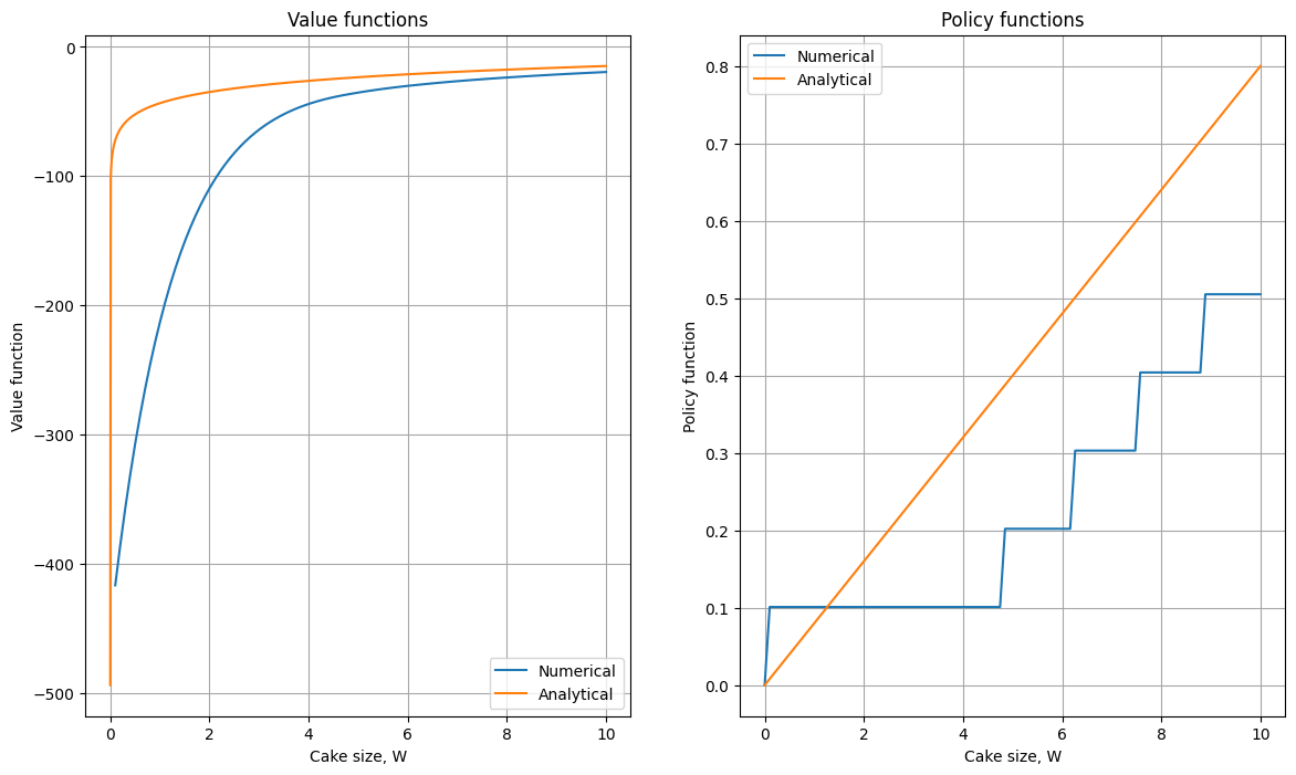
Approach 1: Discretizing continuous choice

• Discretize the continuous state variable \(W\)

• Discretize the continuous choice variable \(c\) as well

Advantage: easy computation of maximum in the Bellman equation (also robustness to local maxima in non-convex problems)

Disadvantage: severe loss of accuracy when choice grid is insufficient

Lets see.

Construct a grid (vector) of cake-sizes \( \vec{W}\in\{0,\dots\overline{W}\} \)

\[ V_{i}(\vec{W})=\max_{0 \le c \le \vec{W}}\{u(c)+\beta V_{i-1}(\vec{W}-c)\} \]

• Compute value and policy function sequentially point-by-point

• May need to compute the value function between grid points \( \Rightarrow \) Interpolation and function approximation

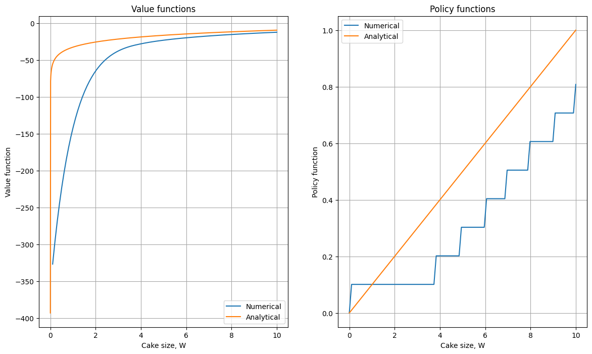
Avoiding interpolation

But we could avoid interpolation by rewriting

\[ V_{i}(\vec{W})=\max_{0 \le \vec{W}' \le \vec{W}}\{u(\vec{W}-\vec{W}')+\beta V_{i-1}(\vec{W}')\} \]

• Can replace \( c \) with \( W_{t+1} \) in Bellman equation so that next period cake size is the decision variable

• Compute value and policy function sequentially point-by-point

• Note that grid \( \vec{W}\in\{0,\dots\overline{W}\} \) is used twice: for state space and for decision space

Can you spot the potential problem?

Show code cell source

Hide code cell source

m1 = cake_ongrid(beta=0.92,Wbar=10,ngrid=100)
check_analytic(m1)

With secondary choice grid

Clearly, reusing the same grid for state and choice is a bad idea which leads to a drastic loss of accuracy!

We should control for grid over state space separately from the discretization of the choice variables to increase accuracy.

• Discretize state space with \(\vec{W}\in\{0,\dots\overline{W}\}\)

• Discretize decision space with \(\vec{D}\in\{0,\dots\overline{D}\}\)

• We could set \(\overline{D}=\overline{W}\), but much better is to use \(\overline{D} = \vec{W}_j\) for each point of the state space \(\vec{W}_j\) to explicitly respect the \(0 \le c \le W\) constraint (controlled by the optim_ch argument in the example)

\[ V_{i}(\vec{W})=\max_{c \in \vec{D}}\{u(c)+\beta V_{i-1}(\vec{W}-c)\} \]

Complication: have to interpolate the computed on the previous iteration value and policy functions between the points of the state grid.

Show code cell source

Hide code cell source

m2 = cake_discretized(beta=0.9,Wbar=10,ngrid=100,nchgrid=100,optim_ch=False)
m3 = cake_discretized(beta=0.9,Wbar=10,ngrid=100,nchgrid=100,optim_ch=True)
check_analytic(m2)
check_analytic(m3)

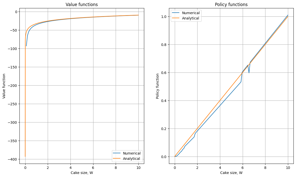
Clear improvement in the accuracy of the solution, but still ways to go!

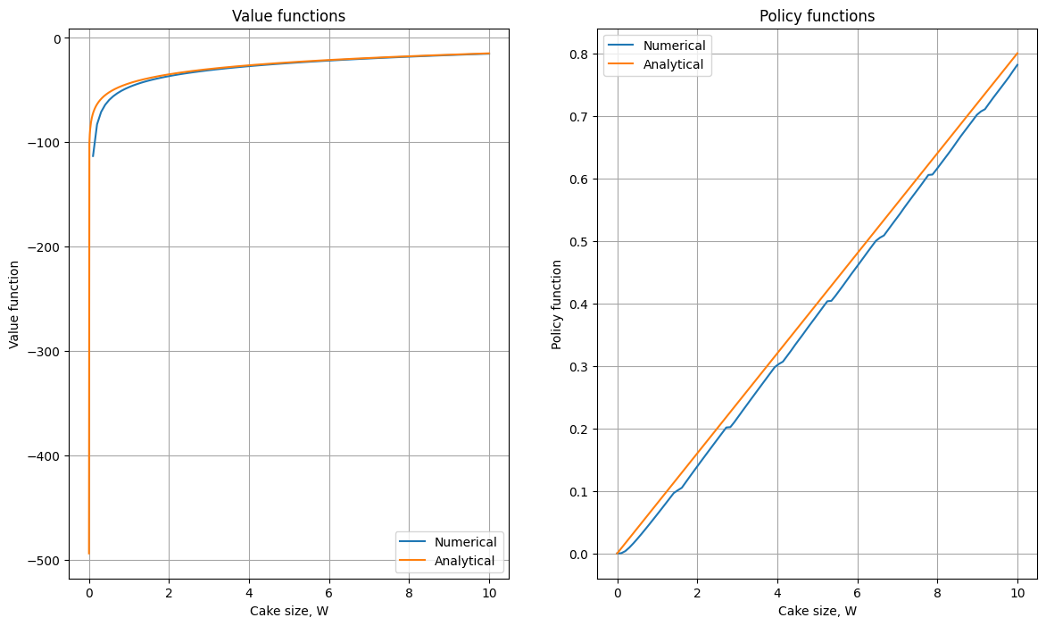
How to increase the accuracy?

• increase the number of grid points, both in state space and especially in choice space

• optimize the use of the grid points in the choice space by accounting for the constraints of the model

• relocate the state grid points towards the ares of higher curvature of the value function

• use a more sophisticated approximation technique

Approach 2: Repeated numerical optimization

Attack the optimization problem directly and run the optimizer to solve

\[ \max_{0 \le c \le \vec{W}}\{u(c)+\beta V_{i-1}(\vec{W}-c)\} \]

Advantage: potentially much more accurate solution

Disadvantages:

• optimization requires an iterative method run in every point of the state space grid in each time period \(\Rightarrow\) potentially very slow approach

• alogorithm has to be robust may fail to converge or get stuck in local maxima

• the latter is a severe problem in complicated models (for example, non-convex problems)

Thoughts on appropriate numerical optimization method

• For Newton we would need first and second derivatives of \(V_{i-1}\), which is itself only approximated on a grid, so no go..

• The problem is bounded, so constrained optimization method is needed

• Bisections should be considered

• Other derivative free methods?

• Quasi-Newton method with bounds?

The Python implementation can make use of scipy.optimize.minimize_scalar(method=’bounded’) which is the Brent method to find a local minimum.

Show code cell source

Hide code cell source

m4 = cake_continuous (beta=0.92,Wbar=10,ngrid=100,tol_bellman=1e-8)
check_analytic(m4)

Approach 3: Endogenous gridpoint method

By far the best available solution method for the consumption-savings model!

• fastest and most accurate solution methods for particular problems with continuous choice

• finite and infinite horizon, discrete time

• applicable to many other important problems

• has multiple generalizations which are applicable to a larger class of problems

Main idea: avoid the numerical optimization step in the Bellman equation by constructing the grid of the state variable endogenously based on the first order condition of the problem

In other words, EGM = guess the optimal consumption, and find the point in the state space where the guessed value is indeed optimal.

Euler equation

The first order condition (FOC) for the cake eating problem is given by

\[ \frac{1}{c_{t}} + \beta \frac{\partial V(W_{t+1})}{\partial W_{t+1}} \frac{\partial W_{t+1}}{\partial c_{t}} = 0 \]

\[ \frac{1}{c_{t}} = \beta \frac{\partial V(W_{t+1})}{\partial W_{t+1}} \]

In the same time by the envelope theorem we have

\[ \frac{\partial V(W_{t})}{\partial W_{t}} = \beta \frac{\partial V(W_{t+1})}{\partial W_{t+1}} \frac{\partial}{\partial W_{t}}(W_{t}-c_{t}) \]

Combining the two equations we realize that \(\frac{1}{c_{t}} = \frac{\partial V(W_{t})}{\partial W_{t}}\), which obviously holds at any \(t\). Thus, we get the Euler equation which characterizes the optimal intertemporal allocation of cake consumption

\[ \frac{1}{c_{t}} = \frac{\beta}{c_{t+1}} \]

Given the optimal consumption level in the next period \(c_{t+1}\), we can compute the optimal consumption in the current period \(c_{t}\) as \(c_{t} = c_{t+1} / \beta\).

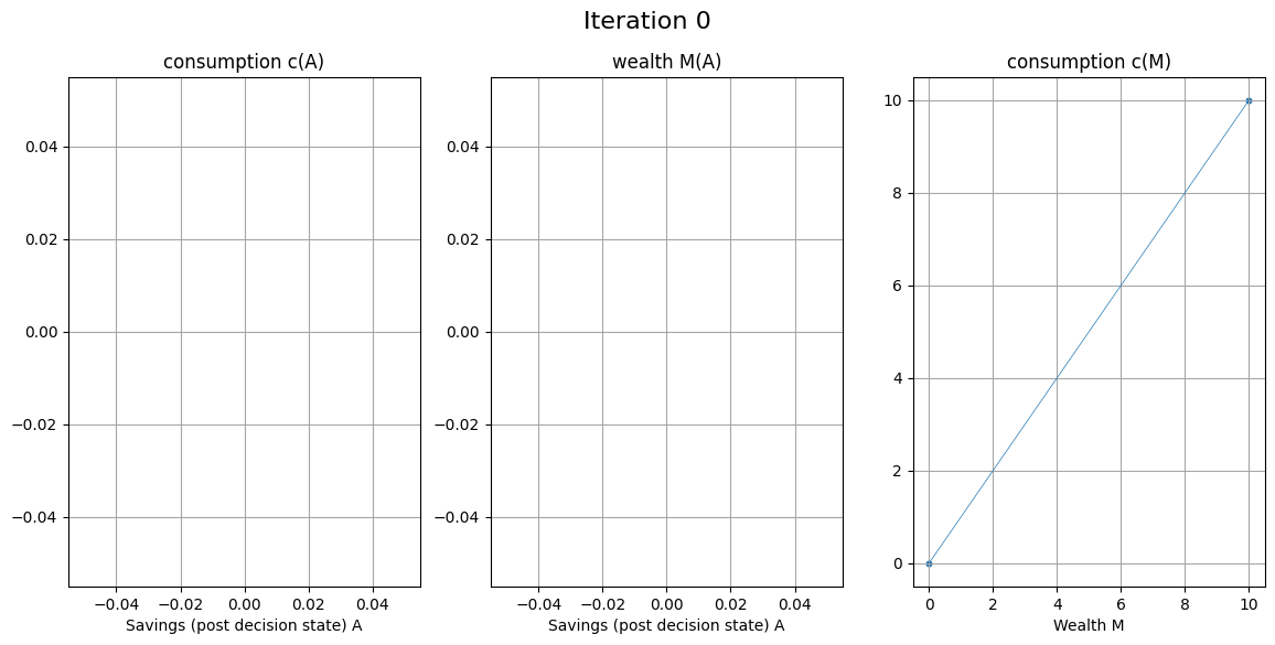
Full EGM algorithm

1. Set a grid on (discretize) post-decision state \(A = W-c\) instead of state \(W\) (how much cake is left for the future after today’s consumption)

2. Set the initial policy \(c_0(W) = W\) defined over two points \(W \in \{0,\bar{W}\}\) provided linear interpolation in used

3. Increment iteration counter \(i\) (initialized to 0)

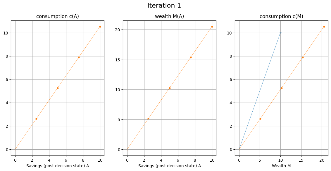
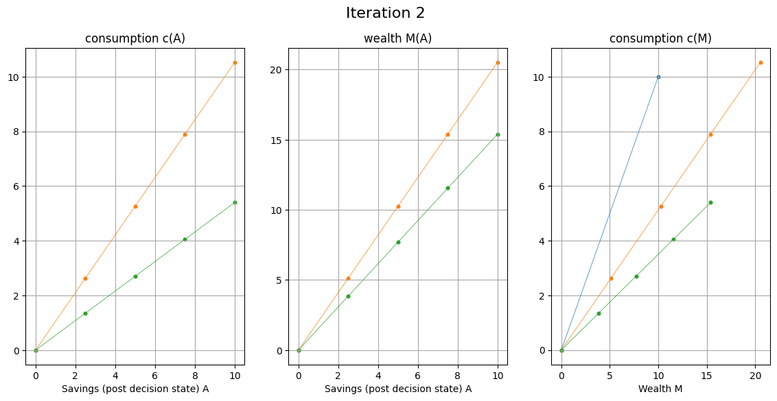
4. For each point \(A_j\) on the grid over \(A\) do:

• Realize that the next period cake size is given by \(W'_j = A_j\)

• Compute the optimal consumption in the next period using the previous iteration policy function \(c_{i-1}(A_j)\)

• Using the (analytically inverted) Euler equation, compute the optimal level of consumption in the current period \(c_j\)

• Compute the endogenous state point \(W_j = A_j + c_j\)

1. Combine all computed endogenous points in the state space \(W_j\), and their corresponding consumption levels \(c_j\) to build the updated policy function \(c_i(W)\)

2. Return to step 3, unless convergence achieved (policy functions \(c_i(W)\) and \(c_{i-1}(W)\) are within given tolerance)

Advantages:

• no root-finding operations, direct computation instead \( \rightarrow \) fast

• Euler equation holds in the generated endogenous state points \( \rightarrow \) accurate

Disadvantages: applies only to particular class of problems

Consumption-savings model (Deaton-Phelps-Carroll)

\[ V(M)=\max_{0 \le c \le M}\big\{u(c)+\beta V\big(\underset{=M'}{\underbrace{R(M-c)+y}}\big)\big\} \]

• What has changed?

New interpretation:

• Wealth in the beginning of the period \(t\) is \(M\)

• Consumption during the period \( t \) is \( 0 \le c \le M \)

• No borrowing is allowed

• Discount factor \( \beta \), time separable utility \( u(c) = \log(c) \)

• Gross return on savings \( R \), (can be stochastic!)

• Constant income \( y \ge 0 \), (can be stochastic!)

This is the cake eating problem when \(R=1\) and \(y=0\)

The stochastic version of the model has to take expectations with respect to the distributions of \(\tilde{R}\) and \(\tilde{y}\) if they are random variables.

\[ V(M)=\max_{0 \le c \le M}\big\{u(c)+\beta \mathbb{E}_{R,y} V\big(\underset{=M'}{\underbrace{\tilde{R}(M-c)+\tilde{y}}}\big)\big\} \]

• we focus on income fluctuations \( \tilde{y} \) and fix \( \tilde{R} \)

• let stochastic income \( \tilde{y} \) follow a log-normal distribution with parameters \( \mu = 0 \) and \( \sigma \) to be specified

• then \( \tilde{y} > 0 \) and \( \mathbb{E}(\tilde{y}) = \exp(\sigma^2/2) \)

• for backward compatibility add \( y=0 \) special case

https://en.wikipedia.org/wiki/Log-normal_distribution

How to compute the expectation?

1. Quadrature methods, best for up to dimension 3-4

2. Monte Carlo integration

• Both methods transform the integral into a weighted sum

• where the terms are the values of the function to be integrated evaluated at certain points (nodes)

• and the weights are determined by the integration method

\[ \int_a^b f(x) dx = \sum_{i=1}^n \omega_i f(x_i) \]

• \( x_i \in [a,b] \) quadrature nodes

• \( \omega_i \) quadrature weights

See lecture 34 in my Foundations of Computational Economics course, and we will see how it is done in the code.

Euler equation for Deaton model

FOC: \( \quad u'(c^\star) - \beta R \mathbb{E}_{y} V'\big(R(M-c^\star)+\tilde{y}\big) = 0 \)

Envelope theorem: \( \quad V'(M) = \beta R \mathbb{E}_{y} V'\big(R(M-c^\star)+\tilde{y}\big) \)

Euler equation:

\[ u'\big(c^\star(M)\big) = \beta R \mathbb{E}_{y} u'\big(c^\star\big(\underset{=M'}{\underbrace{R[M-c^\star(M)]+\tilde{y}}}\big)\big) \]

Let \( A \) denote end-of-period wealth = wealth after consumption, that is savings

Timing of the model:

\[ M \rightarrow c(M) \rightarrow A = M-c(M) \rightarrow M' = R(M-c(M)) + \tilde{y} = RA + \tilde{y} \]

\[ 0 \le c \le M \; \Rightarrow \; 0 \le A = M-c \le M \]

• \( A \) contains all the information needed for the calculation of the expected value function in the next period

• it is sufficient statistic for the current period state and choice

• \( A \) is often referred to as post-decision state

Euler equation with post-decision state can be written as

\[ u'\big(c(M)\big) = \beta R \mathbb{E}_{y} u'\big(c(RA+\tilde{y})\big) \]

• if policy function \( c(M) \) is optimal, then it satisfies the above equation with \( A = M-c(M) \)

• given any policy function \( c(M) \), an updated policy function \( c'(M') \) is given as a parameterized curve

\[\begin{split} \begin{cases} c' = (u')^{-1} \Big( \beta R \mathbb{E}_{y} u'(c\big(RA+\tilde{y})\big) \Big) \\ M' = A + c' \end{cases} \end{split}\]

• where parameter \( A \) ranges over the interval \( (0,M) \)

This is the basis for the EGM algorithm for the consumption-savings model.

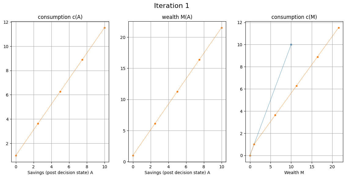
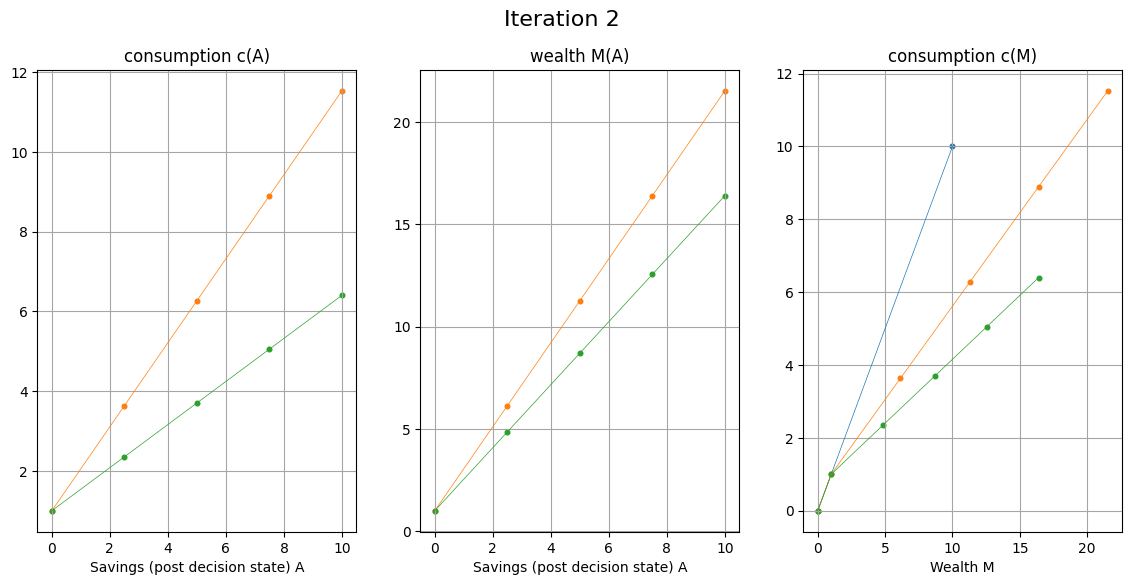
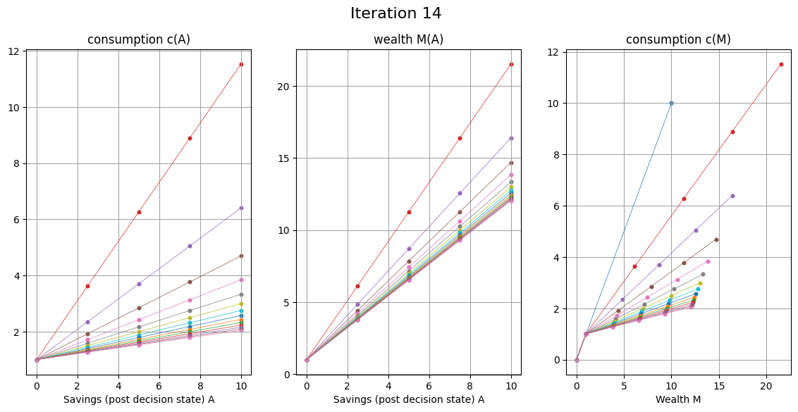
EGM for consumption-savings model

1. Fix grid over \( A \)

2. With given \( c(M) \) for each point on the grid compute

\[\begin{split} \begin{cases} c' = (u')^{-1} \Big( \beta R \mathbb{E}_{y} u'(c\big(RA+\tilde{y})\big) \Big) \\ M' = A + c' \end{cases} \end{split}\]

1. Build the returned policy function \( c'(M) \) as interpolation over computed points \( (M',c') \)

EGM algorithm

1. Set a grid on (discretize) post-decision state \( A \) instead of state \( M \)

2. Set the initial policy \( c_0(M) = M \) defined over two points \( M \in \{0,\bar{M}\} \)

3. Increment iteration counter \( i \) (initialized to 0)

4. For each point \( A_j \) on the grid over \( A \) perform the EGM step and return the corresponding value of consumption \( c_j \) and the endogenous point of wealth \( M_j = A_j+c_j \)

5. Combine all computed endogenous points in the state space \( M_j \), and their corresponding consumption levels \( c_j \) to build the updated policy function \( c_i(M) \)

6. Return to step 3, unless convergence achieved (policy functions \( c_i(M) \) and \( c_{i-1}(M) \) are within given tolerance)

EGM step: Given point \( A_j \) on the grid over \( A \):

1. Compute the next period wealth \( M'_j = RA_j + \tilde{y} \), replacing \( \tilde{y} \) with quadrature points

2. Compute the optimal consumption in the next period in all quadrature points, using the previous iteration policy function \( c_{i-1}(\cdot) \)

3. Compute the marginal utility for each value of consumption, and complete the calculation of the expectation in RHS of Euler equation

4. Using inverse marginal utility function, compute optimal consumption \( c_j \) in current period, corresponding to the point \( A_j \)

5. complete the EGM step by computing endogenous state point \( M_j = A_j + c_j \)

EGM for consumption-savings model

\[ V(M)=\max_{0 \le c \le M}\big\{log(c)+\beta V\big(R(M-c)+y\big)\big\} \]

\[ u'\big(c^\star(M)\big) = \beta R u'\big(c^\star\big(R[M-c^\star(M)]+y\big)\big) \]

\[\begin{split} \begin{cases} c' = (u')^{-1} \Big( \beta R u'(c\big(RA+y)\big) \Big) \\ M' = A + c \end{cases} \end{split}\]

Show code cell source

Hide code cell source

import numpy as np
import matplotlib.pyplot as plt
from scipy import interpolate
%matplotlib inline

beta,R,y = 0.95,1.,0.    # fundamentals (cake eating)
Mbar,ngrid = 10,5        # technical parameters
u = lambda c: np.log(c)  # utility function
mu = lambda c: 1/c       # marginal utility function
imu = lambda u: 1/u      # inverse marginal utility function
A = np.linspace(0,Mbar,ngrid)
c0 = np.array([0,Mbar])
M0 = np.array([0,Mbar])
from itertools import cycle
prop_cycle = plt.rcParams['axes.prop_cycle']
colors = cycle(prop_cycle.by_key()['color'])
fig, ax = plt.subplots(1,3,figsize=(14,6))
for axi in ax:
    axi.grid(visible=True, which='both', color='0.65', linestyle='-')
ax[0].set_title('consumption c(A)')
ax[1].set_title('wealth M(A)')
ax[2].set_title('consumption c(M)')
ax[0].set_xlabel('Savings (post decision state) A')
ax[1].set_xlabel('Savings (post decision state) A')
ax[2].set_xlabel('Wealth M')
def plot_iter(a,m,c,suptitle='',color=None):
    if color is None:
      color = next(colors)
    ax[0].plot(a,c,linewidth=0.5,c=color)
    ax[1].plot(a,m,linewidth=0.5,c=color)
    ax[2].plot(m,c,linewidth=0.5,c=color)
    ax[0].scatter(a,c,s=11,c=color)
    ax[1].scatter(a,m,s=11,c=color)
    ax[2].scatter(m,c,s=11,c=color)
    fig.suptitle(suptitle,fontsize=16)
    return fig,color

_,cl0 = plot_iter(np.full(2,np.nan),M0,c0,'Iteration 0')
plt.show()

Show code cell source

Hide code cell source

fig, ax = plt.subplots(1,3,figsize=(14,6))
for axi in ax:
    axi.grid(visible=True, which='both', color='0.65', linestyle='-')
ax[0].set_title('consumption c(A)')
ax[1].set_title('wealth M(A)')
ax[2].set_title('consumption c(M)')
ax[0].set_xlabel('Savings (post decision state) A')
ax[1].set_xlabel('Savings (post decision state) A')
ax[2].set_xlabel('Wealth M')
plot_iter(np.full(2,np.nan),M0,c0,'Iteration 0',cl0)

# Iteration 1
policy = interpolate.interp1d(M0,c0,kind='slinear',fill_value="extrapolate")  # interpolation function for policy
M1 = np.full(ngrid,np.nan)
c1 = np.full(ngrid,np.nan)
for j,aj in enumerate(A):
    Mpr = max(R*aj+y,1e-10)        # next period wealth
    cpr = policy(Mpr)              # next period consumption
    c1[j] = imu( beta*R*mu(cpr) )  # inverse Euler
    M1[j] = aj + c1[j]             # endogenous wealth
_,cl1 = plot_iter(A,M1,c1,'Iteration 1')
plt.show()

Show code cell source

Hide code cell source

fig, ax = plt.subplots(1,3,figsize=(14,6))
for axi in ax:
    axi.grid(visible=True, which='both', color='0.65', linestyle='-')
ax[0].set_title('consumption c(A)')
ax[1].set_title('wealth M(A)')
ax[2].set_title('consumption c(M)')
ax[0].set_xlabel('Savings (post decision state) A')
ax[1].set_xlabel('Savings (post decision state) A')
ax[2].set_xlabel('Wealth M')
plot_iter(np.full(2,np.nan),M0,c0,'Iteration 0',cl0)
plot_iter(A,M1,c1,'Iteration 1',cl1)

# Iteration 2
policy = interpolate.interp1d(M1,c1,kind='slinear',fill_value="extrapolate")  # interpolation function for policy
M2 = np.full(ngrid,np.nan)
c2 = np.full(ngrid,np.nan)
for j,aj in enumerate(A):
    Mpr = max(R*aj+y,1e-10)        # next period wealth
    cpr = policy(Mpr)              # next period consumption
    c2[j] = imu( beta*R*mu(cpr) )  # inverse Euler
    M2[j] = aj + c2[j]             # endogenous wealth
_,cl2=plot_iter(A,M2,c2,'Iteration 2')
plt.show()

Corner solutions in EGM

• So far only covered the interior solutions where the Euler equation holds

• What about the restriction \( 0 \le c \le M \) which is equivalent to \( 0 \le A \le M \)?

1. By choosing the grid on \( A \) to respect the constraint \( 0 \le A \le M \) EGM only implements interior solutions

2. Corner solutions must be added with an additional provisions in the code

Lower bound on consumption

• \( c \ge 0 \) is never binding if utility function satisfies

\[ \lim_{c \rightarrow 0} u(c) = -\infty \]

• all our usual utility functions like \( \log(c) \) or CRRA utility \( \frac{c^\lambda - 1}{\lambda} \) satisfy this condition

Upper bound on consumption

• If \( c \le M \) is binding, then \( A=0 \), can be computed directly

Proposition If utility function \( u(c) \) in the consumption-savings model is monotone and concave, then end-of-period wealth \( A=M-c \) is non-decreasing in M.

• Let \( M_0 = (u')^{-1} \Big( \beta R \mathbb{E}_{y} u'(c(\tilde{y})\big) \Big) \) denote the point that corresponds to \( A=0 \)

• Due to the proposition, for all \( M<M_0 \) the end of period wealth must be zero, and thus optimal consumption \( c=M \) is the corner solution

• To implement this in the code, we just need to add a 45 degrees segment to the consumption function below \(M_0\)

Show code cell source

Hide code cell source

import numpy as np
import matplotlib.pyplot as plt
from scipy import interpolate

beta,R,y = 0.95,1.05,1   # fundamentals
Mbar,ngrid = 10,5        # technical parameters
u = lambda c: np.log(c)  # utility function
mu = lambda c: 1/c       # marginal utility function
imu = lambda u: 1/u      # inverse marginal utility function

A = np.linspace(0,Mbar,ngrid)  # What are the bounds of A?
c0 = np.array([0,Mbar])
M0 = np.array([0,Mbar])

from itertools import cycle
prop_cycle = plt.rcParams['axes.prop_cycle']
colors = cycle(prop_cycle.by_key()['color'])

fig, ax = plt.subplots(1,3,figsize=(14,6))
for axi in ax:
    axi.grid(visible=True, which='both', color='0.65', linestyle='-')
ax[0].set_title('consumption c(A)')
ax[1].set_title('wealth M(A)')
ax[2].set_title('consumption c(M)')
ax[0].set_xlabel('Savings (post decision state) A')
ax[1].set_xlabel('Savings (post decision state) A')
ax[2].set_xlabel('Wealth M')

_,cl0=plot_iter(np.full(2,np.nan),M0,c0,'Iteration 0')
plt.show()

Show code cell source

Hide code cell source

# Iteration function
Aex = np.full(ngrid+1,np.nan)
Aex[1:] = A
def iter(M0,c0,iter):
    policy = interpolate.interp1d(M0,c0,kind='slinear',fill_value="extrapolate")  # interpolation function for policy
    M1 = np.full(ngrid+1,np.nan)
    c1 = np.full(ngrid+1,np.nan)
    M1[0] = c1[0] = 0              # add one point at the origin!
    for j,aj in enumerate(A):
        Mpr = max(R*aj+y,1e-10)    # next period wealth
        cpr = policy(Mpr)          # next period consumption
        c = imu( beta*R*mu(cpr) )  # inverse Euler
        M = aj + c                 # endogenous wealth
        M1[j+1] = M                # save to array
        c1[j+1] = c
    _,cl = plot_iter(Aex,M1,c1,f'Iteration {iter}')
    return M1,c1,cl

fig, ax = plt.subplots(1,3,figsize=(14,6))
for axi in ax:
    axi.grid(visible=True, which='both', color='0.65', linestyle='-')
ax[0].set_title('consumption c(A)')
ax[1].set_title('wealth M(A)')
ax[2].set_title('consumption c(M)')
ax[0].set_xlabel('Savings (post decision state) A')
ax[1].set_xlabel('Savings (post decision state) A')
ax[2].set_xlabel('Wealth M')

plot_iter(np.full(2,np.nan),M0,c0,'Iteration 0',cl0)
M1,c1,cl1 = iter(M0,c0,1)
plt.show()

Show code cell source

Hide code cell source

fig, ax = plt.subplots(1,3,figsize=(14,6))
for axi in ax:
    axi.grid(visible=True, which='both', color='0.65', linestyle='-')
ax[0].set_title('consumption c(A)')
ax[1].set_title('wealth M(A)')
ax[2].set_title('consumption c(M)')
ax[0].set_xlabel('Savings (post decision state) A')
ax[1].set_xlabel('Savings (post decision state) A')
ax[2].set_xlabel('Wealth M')

plot_iter(np.full(2,np.nan),M0,c0,'Iteration 0',cl0)
plot_iter(Aex,M1,c1,'Iteration 1',cl1)
M2,c2,cl2 = iter(M1,c1,2)
plt.show()

Show code cell source

Hide code cell source

fig, ax = plt.subplots(1,3,figsize=(14,6))
for axi in ax:
    axi.grid(visible=True, which='both', color='0.65', linestyle='-')
ax[0].set_title('consumption c(A)')
ax[1].set_title('wealth M(A)')
ax[2].set_title('consumption c(M)')
ax[0].set_xlabel('Savings (post decision state) A')
ax[1].set_xlabel('Savings (post decision state) A')
ax[2].set_xlabel('Wealth M')
plot_iter(np.full(2,np.nan),M0,c0,'Iteration 0',cl0)
M,c = M0,c0
for i in range(1,15):
    M,c,cl = iter(M,c,i)
plt.show()

Class of models solvable by EGM

• finite and infinite horizon dynamic models with continuous choice

• strictly concave monotone and differentiable utility function (with analytic inverse marginal)

• one continuous state variable (wealth) and one continuous choice variable (consumption)

• particular structure of the law of motion for state variables (intertemporal budget constraint)

• occasionally binding borrowing constraints

• can also easily allow additional quasi-exogenous state variables (with motion rules dependent on \( A \) and not \( M \) or \( c \))

Rather small class, although many important models in micro and macro economics are included

Generalizations for multiple dimensions

• Hard because irregular grids in multiple dimensions

• 📖 Barillas and Fernández-Villaverde [2007] “A Generalization of the Endogenous Grid Method”, Jounrnal of Economic Dynamics and Control

• 📖 Ludwig and Schön [2018] “Endogenous Grids in Higher Dimensions: Delaunay Interpolation and Hybrid Methods”, Computational Economics

• 📖 White [2015] “The Method of Endogenous Gridpoints in Theory and Practice”, Journal of Economic Dynamics and Control

• 📖 Iskhakov [2015] “Multidimensional endogenous gridpoint method: solving triangular dynamic stochastic optimization problems without root-finding operations” + Corrigendum, Economics Letters

• 📖 Lujan [n.d.] “EGMn: The Sequential Endogenous Grid Method” “

Generalizations for non-convex problems

• Hard because Euler equation is not a sufficient condition any longer!

• EGM recovers all solutions of thet Euler equation, thus all local maxima, but additional steps are needed to filter out the suboptimal solutions

• Still avoids root-finding operations, thus remains much faster than any alternative methods (which also have to deal with multiple local maxima)

• 📖 Fella [2014] A Generalized Endogenous Grid Method for Non-Smooth and Non-Concave Problems”, Review of Economic Dynamics

• 📖 Iskhakov et al. [2017] “The endogenous grid method for discrete-continuous dynamic choice models with (or without) taste shocks”, Quantitative Economics

• 📖 Druedahl and Jørgensen [2017] “A general endogenous grid method for multi-dimensional models with non-convexities and constraints”, Journal of Economic Dynamics and Control

But if you model fits EGM framework, use it! It is by far the best available method for such problems!

References and Additional Resources

• 📖 Carroll [2006] “The method of endogenous gridpoints for solving dynamic stochastic optimization problems”, Economics Letters

• 📖 Iskhakov et al. [2017] “The endogenous grid method for discrete-continuous dynamic choice models with (or without) taste shocks”, Quantitative Economics

• 📖 Druedahl and Jørgensen [2017] “A general endogenous grid method for multi-dimensional models with non-convexities and constraints”, Journal of Economic Dynamics and Control

• Youtube video exlpainer of Brent’s optimization method by Oscar Veliz https://www.youtube.com/watch?v=BQm7uTYC0sg