📖 Method of simulated moments (MSM) for model estimation

⏱ | words

References

Next step after solver and simulator are debugged

Estimate model parameters from simulated data?

• study the implications of theoretical assumptions of various models and theories

• run numerical simulations of optimal decisions and policies (for particular values or ranges of values of model parameters)

But the ultimate goal is to match the model to the actually observed data, and:

• quantify of the effects of various parts of the theoretical setup

• perform counterfactual experiments simulating the behavior of the decision maker in hypothetical policy regimes

• support or falsify theoretical results by examining their fit to the observed data

Estimation vs. calibration

What is the difference? Sometimes the terms are used interchangeably

• Standard errors of estimates (measure of variability of the estimation results)

• Study of identification (to make sure that only a single parameter values can maximize the statistical criterion and explain the data)

Calibration exercises often skip these steps, even if employing algorithmic search of best parameters to fit the model to the data.

Applications of estimation sometimes estimate only a subset of parameters, treating other as fixed, similar to calibration with parameter values from the literature.

Workflow of structural estimation

1. Theoretical model development (what is of interest?)

2. Practical specification/implementation issues

3. Solving the model (method + implementation in the code)

4. Understanding how the model works

5. Estimation: running the statistical procedure

6. Validation (assessing in-sample and out-of-sample performance)

7. Policy experiments, counterfactual simulations

Example

Stochastic consumption-savings model

\[ V(M)=\max_{0 \le c \le M}\big\{u(c)+\beta V\big(\underset{=M'}{\underbrace{R(M-c)+y}}\big)\big\} \]

• solver to compute the optimal policy function for given parameter values

• simulator to simulate data for given parameter values (and model solution)

Need:

• estimation procedure to find the “best” parameter values to fit the model to the observed data

• counterfactual simulation program to use the estimated model for policy experiments

Understanding how the model works

1. Solve the model for a set of parameter values

2. Simulated data from the model

3. Does it make (economic) sense?

4. Repeat (many-many times)

• may take a lot of time to convince yourself that the code does not have bugs

• unexpected/surprising results still appear? Making research progress!

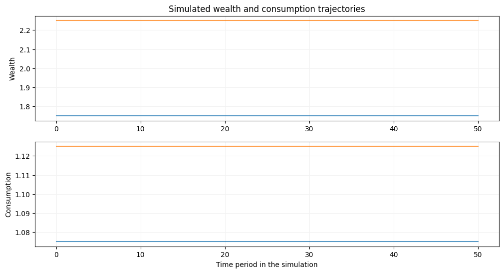
# deterministic model with βR=1 and y=1
m = deaton(beta=0.9,R=1/0.9,ngrid=100,nchgrid=250,sigma=1e-10,nquad=2)
m.solve_egm(tol=1e-10)
init_wealth, T = [1.75,2.25], 50
m.simulator(init_wealth=init_wealth,T=T,seed=2020)
plt.show()

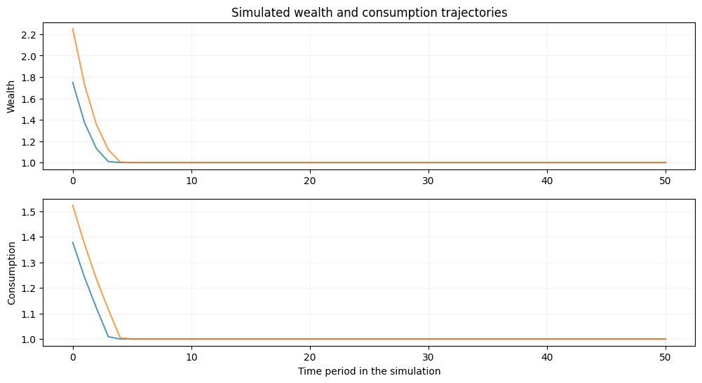
# deterministic model with R=1 and y=1
m = deaton(beta=0.9,R=1.0,ngrid=100,nchgrid=250,sigma=1e-10,nquad=2)
m.solve_egm(tol=1e-10)
init_wealth, T = [1.75,2.25], 50
m.simulator(init_wealth=init_wealth,T=T,seed=2020)
plt.show()

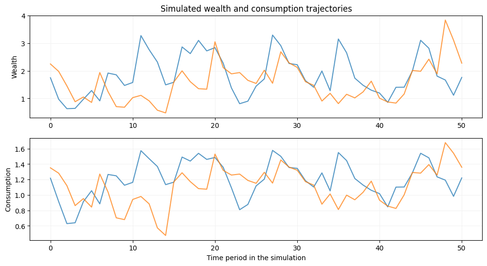
# two stochastic models with different income variance
m1 = deaton(beta=0.9,R=1.05,ngrid=100,nchgrid=250,sigma=0.5)
m2 = deaton(beta=0.9,R=1.05,ngrid=100,nchgrid=250,sigma=0.85)
m1.solve_egm(tol=1e-10)
m2.solve_egm(tol=1e-10)
init_wealth, T = [1.75,2.25], 50
m1.simulator(init_wealth=init_wealth,T=T,seed=2020)
m2.simulator(init_wealth=init_wealth,T=T,seed=2020)
plt.show()

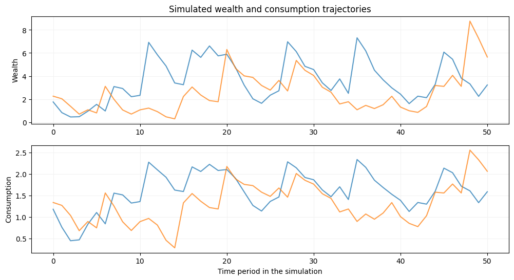
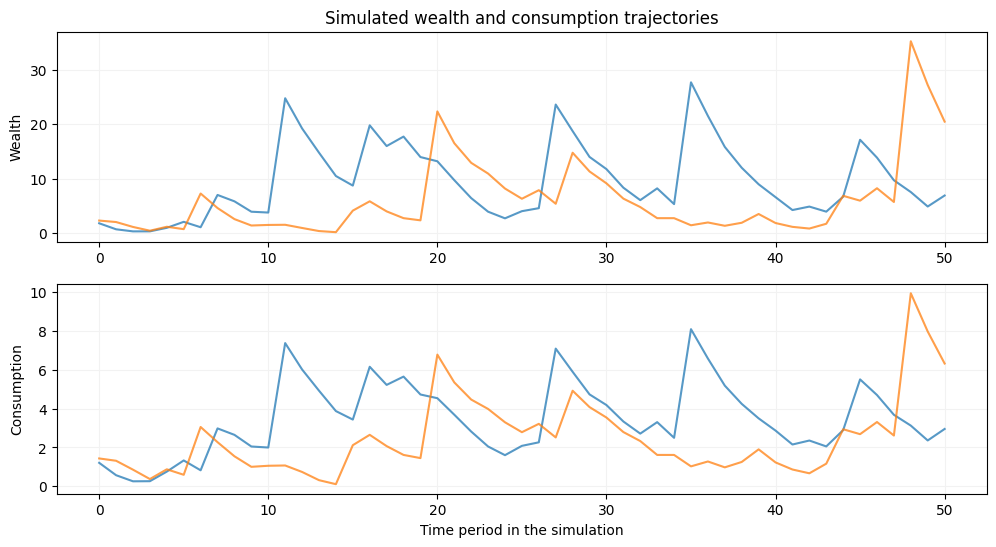
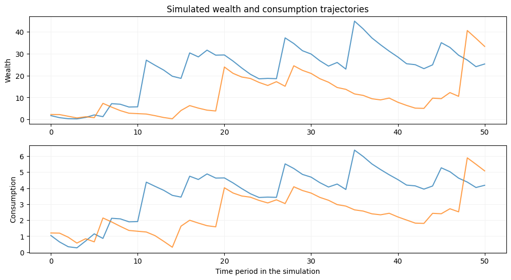
# two stochastic models with different dicount coefficients
m1 = deaton(beta=0.85,R=1.05,ngrid=100,nchgrid=250,sigma=1.5)
m2 = deaton(beta=0.95,R=1.05,ngrid=100,nchgrid=250,sigma=1.5)
m1.solve_egm(tol=1e-10)
m2.solve_egm(tol=1e-10)
init_wealth, T = [1.75,2.25], 50
m1.simulator(init_wealth=init_wealth,T=T,seed=2020)
m2.simulator(init_wealth=init_wealth,T=T,seed=2020)
plt.show()

Method of simulated moments

• we have seen how changing parameters is reflected in changes in the simulated wealth and consumption profiles

• imagine we have data on observed consumption or wealth profiles for a sample of people, or even some aggregate data on consumption or wealth

• then we can find parameters of the model that would induce the simulated data to reflect the observed profiles, or some descriptive statistics (moments) of these profiles

Simulated moments

The idea of directly matching the moments from the model to the observed ones leads to the method of moments estimator

• Method of moments: # of parameters = # of moments to match, system of equations

• Generalized method of moments (GMM): # of parameters < # of moments, minimize the distance between the data moments and theoretical moments

• Method of simulated moments (MSM): using simulations to compute the theoretical moments

Definition of MSM estimator

\[ \hat{\theta}_{MSM}(W) = \arg\min_{\theta \in \Theta} \, e(\tilde{x},x|\theta) \, W e(\tilde{x},x|\theta)^{T} \]

• \( \theta \in \Theta \) is parameter space

• \( e(\tilde{x},x|\theta) \) is the row-vector of \( K \) moment conditions

• \( W \) is the \( K \times K \) weighting matrix

• \( x \) and \( \tilde{x} \) is observed and simulated data

Moments and moment conditions

\[ e(\tilde{x},x|\theta) = \big(e^1(\tilde{x},x|\theta),\dots,e^K(\tilde{x},x|\theta) \big) \]

\[ e^k(\tilde{x},x|\theta) = m^k(x) - m^k(\tilde{x}|\theta) \]

• \( m^k(\cdot) \) is the \( k \)-th moment generating function

• \( m^k(x) \) are empirical moments (computed from the observed data)

• \( m^k(\tilde{x}|\theta) \) are the simulated moments (computed from the simulated data using parameter values \( \theta \))

Theory of MSM

📖 McFadden [1989] “A method of simulated moments for estimation of discrete response models without numerical integration”, Econometrica

📖 Pakes and Pollard [1989] “Simulation and the Asymptotics of Optimization Estimators”, Econometrica

📖 Lee and Ingram [1991] “Simulation estimation of time-series models”, Journal of Econometrics

📖 Duffie and Singleton [1993] “Simulated moments estimation of Markov models of asset”, Econometrica

Statistical properties of MSM estimator

1. \( \hat{\theta}_{MSM}(W) \) is consistent with any weighting matrix \( W \)

2. \( \hat{\theta}_{MSM}(W) \) is asymptotically normal \( \hat{\theta}_{MSM}(W) \sim N(0,\Sigma) \)

Variance-covariance matrix of the estimate

\[ \hat{\Sigma} = (1+\tfrac{1}{\tau})(D^{T} W D)^{-1} D^{T}W \hat{S} W D (D^{T}WD)^{-1} \]

• \( W \) is weighting matrix

• \( D = \partial e(\tilde{x},x|\theta) \big/ \partial \theta \) is the Jacobian matrix of moment conditions, computed at consistent estimate \( \theta \)

• \( S \) is variance-covariance matrix of the moment conditions \( e(\tilde{x},x|\theta) \)

• \( \hat{S} \) is estimate of \( S \), usually computed using simulations as well

• \( \tau \) is the ratio of the simulated to empirical samples sizes

Optimal weighting matrix

• the asymptotic variance of the estimates is minimized when the weighting matrix is given by the inverse of the variance-covariance matrix of the moment conditions (at true value of the parameter)

• the estimate of the variance-covariance matrix of the MSM estimate then becomes

\[ \hat{\Sigma} = (1+\tfrac{1}{\tau})(D^{T} W D)^{-1} \]

• weighting matrix can be estimated using the simulated analog

\[ \hat{W}^\star = \big(\hat{S}\big)^{-1} \]

Weighting matrix in practice

• identity = in the first step of multi-step MSM estimations

• diagonal weighting matrix, ignoring the covariances

• manually chosen weights, i.e. to bring all the moments to the same scale

• using sample variance to downgrade poorly measured empirical moments

• estimated from the moment conditions based on first step consistent estimate

• iteratively updated weighting using multi-step estimating procedure

• Newey-West robust estimate of weighting matrix

• additional model-specific adjustments

Many ways to skin a cat

Choice of moments

• crucial part for MSM estimation = being able to minimize the MSM criterion

• more art than science

• understanding how the model works = understanding what variation is induced in simulated data when parameters change

• selected for estimation \( K \) moments should adequately represent this variation

Practical advantages of MSM

• not data hungry (may match aggregated moments)

• allows to combine different sources of data

• does not rely on the distributional assumptions as much as MLE

• but lacks in efficiency, so standard errors are larger than MLE

• weighting matrix is often simplified in practice due to small sample bias

Widely used method in applied research!

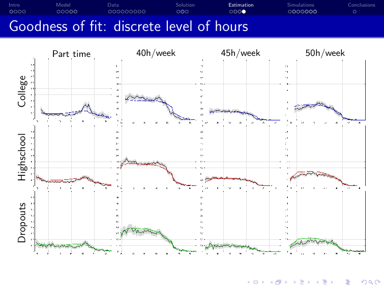
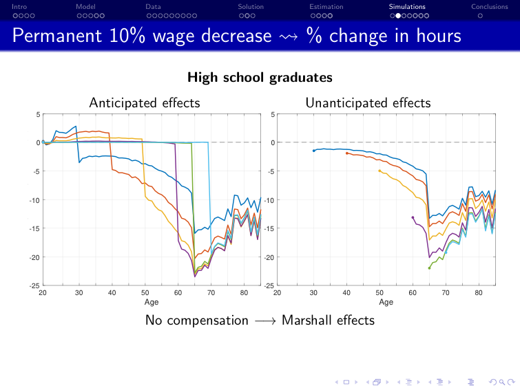
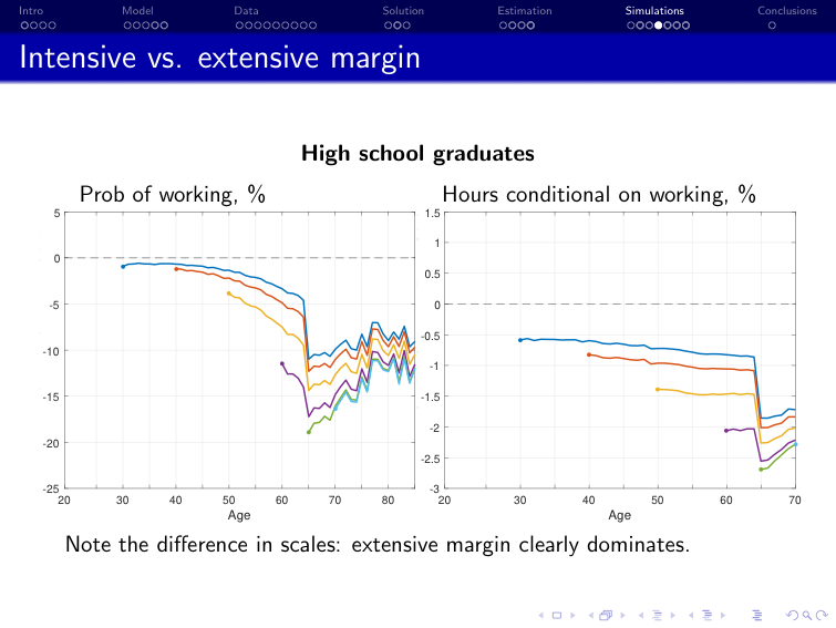
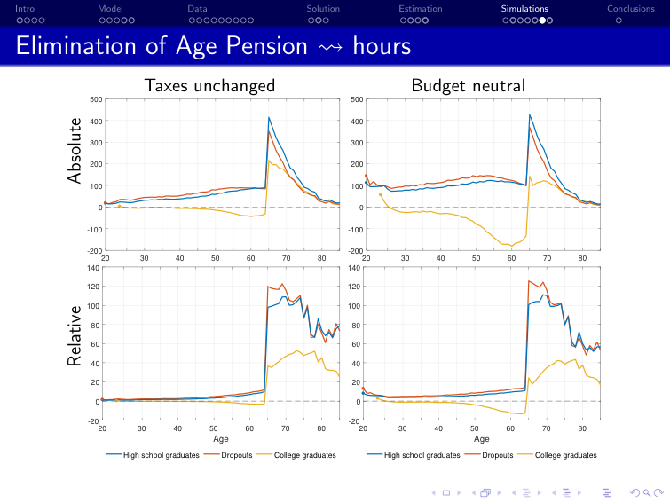
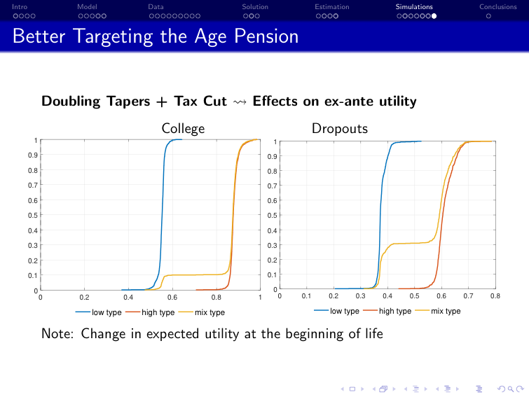
Example of EGM with MSM application in structural econometrics

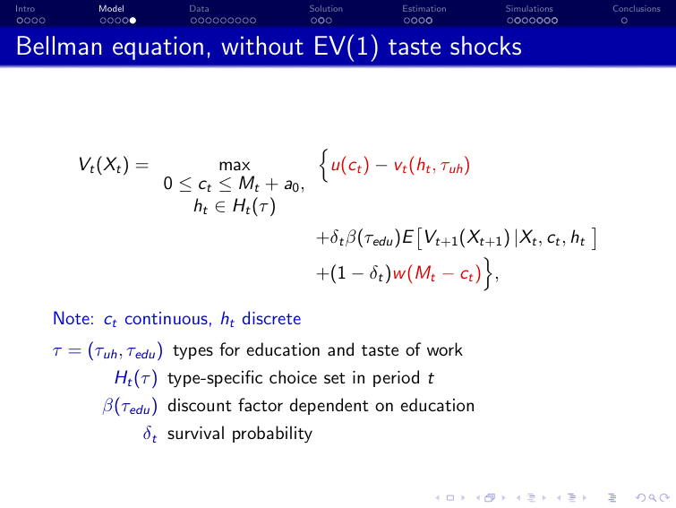
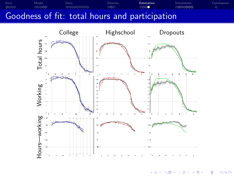
Iskhakov and Keane [2021] “Effects of taxes and safety net pensions on life-cycle labor supply, savings and human capital: The case of Australia”, Journal of Econometrics

• Policy: retargeting of the pension system in Australia

• Structural model: dynamic discrete choice model of labor supply, savings, and human capital

• Equilibrium: none, partial equilibrium analysis with single decision maker (household)

• Estimation: method of simulated moments using Australian survey data on labor supply and income (HILDA)

Download complete slide deck

References and Additional Resources

• 📖 Iskhakov and Keane [2021] “Effects of taxes and safety net pensions on life-cycle labor supply, savings and human capital: The case of Australia”, Journal of Econometrics

• 📖 Adda and Cooper [2023] “Dynamic Economics” pp. 87-89

• 📖 McFadden [1989] “A Method of Simulated Moments for Estimation of Discrete Response Models Without Numerical Integration”, Econometrica

• Youtube video lecture on MSM by Dean Corbae at DSE2024 summer school at the University of Wisconsin Madison https://youtu.be/61KXTkxZb3o?si=TGgQofH069u-7r0G

• Notebook by Richard W Evans on MSM https://notes.quantecon.org/submission/5b3db2ceb9eab00015b89f93